Histograms in Matlab a = A(:); % reshapes matrix A into vector, - - PDF document

9/22/2009 1

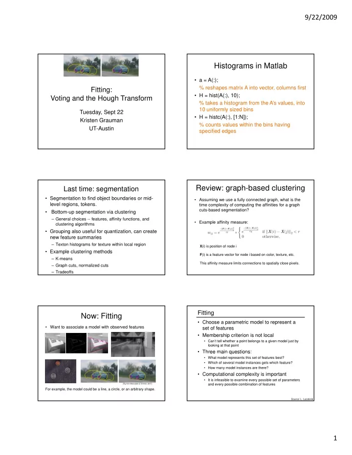
Fitting: Voting and the Hough Transform g g

Tuesday, Sept 22 Kristen Grauman UT-Austin

Histograms in Matlab

• a = A(:);

% reshapes matrix A into vector, columns first

• H = hist(A(:), 10);

% t k hi t f th A’ l i t % takes a histogram from the A’s values, into 10 uniformly sized bins

• H = histc(A(:), [1:N]);

% counts values within the bins having specified edges

Last time: segmentation

• Segmentation to find object boundaries or mid-

level regions, tokens.

• Bottom-up segmentation via clustering

– General choices -- features, affinity functions, and clustering algorithms

• Grouping also useful for quantization, can create

new feature summaries

– Texton histograms for texture within local region

• Example clustering methods

– K-means – Graph cuts, normalized cuts – Tradeoffs

Review: graph-based clustering

• Assuming we use a fully connected graph, what is the

time complexity of computing the affinities for a graph cuts-based segmentation?

• Example affinity measure:

X(i) is position of node i F(i) is a feature vector for node i based on color, texture, etc. This affinity measure limits connections to spatially close pixels.

Now: Fitting

• Want to associate a model with observed features

[Fig from Marszalek & Schmid, 2007]

For example, the model could be a line, a circle, or an arbitrary shape.

Fitting

• Choose a parametric model to represent a

set of features

• Membership criterion is not local
• Can’t tell whether a point belongs to a given model just by

looking at that point

• Three main questions:

ee a quest o s

• What model represents this set of features best?
• Which of several model instances gets which feature?
• How many model instances are there?
• Computational complexity is important
• It is infeasible to examine every possible set of parameters

and every possible combination of features

Source: L. Lazebnik

9/22/2009 2

Example: Line fitting

• Why fit lines?

Many objects characterized by presence of straight lines

• Wait, why aren’t we done just by running edge detection?
• Extra edge points (clutter),

multiple models:

– which points go with which line, if any?

• Only some parts of each line

Difficulty of line fitting

detected, and some parts are missing:

– how to find a line that bridges missing evidence?

• Noise in measured edge

points, orientations:

– how to detect true underlying parameters?

Fitting lines

• Given points that belong to a line, what

is the line?

Forsyth & Ponce 15.2.1

Assuming all the points that belong to a line are known, can solve for line parameters that yield minimal error.

Fitting lines

• Given points that belong to a line, what

is the line?

• How many lines are there?
• Which points belong to which lines?

Voting

• It’s not feasible to check all combinations of features by

fitting a model to each possible subset.

• Voting is a general technique where we let the features

vote for all models that are compatible with it.

– Cycle through features cast votes for model parameters Cycle through features, cast votes for model parameters. – Look for model parameters that receive a lot of votes.

• Noise & clutter features will cast votes too, but typically

their votes should be inconsistent with the majority of “good” features.

• Ok if some features not observed, as model can span

multiple fragments.

Fitting lines

• Given points that belong to a line, what

is the line?

• How many lines are there?
• Which points belong to which lines?
• Hough Transform is a voting
• Hough Transform is a voting

technique that can be used to answer all of these questions. Main idea:

• 1. Record vote for each possible line
• n which each edge point lies.
• 2. Look for lines that get many votes.

9/22/2009 3

Finding lines in an image: Hough space

x y m b m0 b0

Connection between image (x,y) and Hough (m,b) spaces

• A line in the image corresponds to a point in Hough space
• To go from image space to Hough space:

– given a set of points (x,y), find all (m,b) such that y = mx + b

image space Hough (parameter) space

Slide credit: Steve Seitz

Finding lines in an image: Hough space

x y m b x0 y0

Connection between image (x,y) and Hough (m,b) spaces

• A line in the image corresponds to a point in Hough space
• To go from image space to Hough space:

– given a set of points (x,y), find all (m,b) such that y = mx + b

• What does a point (x0, y0) in the image space map to?

image space Hough (parameter) space

– Answer: the solutions of b = -x0m + y0 – this is a line in Hough space

Slide credit: Steve Seitz

Finding lines in an image: Hough space

x y m b x0 y0

b = –x1m + y1 (x0, y0) (x1, y1)

What are the line parameters for the line that contains both (x0, y0) and (x1, y1)?

• It is the intersection of the lines b = –x0m + y0 and

b = –x1m + y1

image space Hough (parameter) space

Finding lines in an image: Hough algorithm

x y m b

How can we use this to find the most likely parameters (m,b) for the most prominent line in the image space?

• Let each edge point in image space vote for a set of

possible parameters in Hough space

• Accumulate votes in discrete set of bins; parameters with

the most votes indicate line in image space. image space Hough (parameter) space

Polar representation for lines

: perpendicular distance from line to origin

d

[0,0] θ

x

Issues with usual (m,b) parameter space: can take on infinite values, undefined for vertical lines.

: angle the perpendicular makes with the x-axis

Point in image space sinusoid segment in Hough space

d y x = − θ θ sin cos

θ

d y

Hough transform algorithm

Using the polar parameterization: Basic Hough transform algorithm

• 1. Initialize H[d, θ]=0
• 2. for each edge point I[x,y] in the image

H: accumulator array (votes)

d

d y x = − θ θ sin cos

for θ = 0 to 180 // some quantization H[d, θ] += 1

• 3. Find the value(s) of (d, θ) where H[d, θ] is maximum
• 4. The detected line in the image is given by

Hough line demo

θ

Time complexity (in terms of number of votes per pt)?

Source: Steve Seitz

θ θ sin cos y x d − =

θ θ sin cos y x d − =

9/22/2009 4

d y

Example: Hough transform for straight lines

Image space edge coordinates Votes

θ x Bright value = high vote count Black = no votes

Example: Hough transform for straight lines

Circle : Square :

Example: Hough transform for straight lines

Showing longest segments found

Impact of noise on Hough

y d

Image space edge coordinates Votes

θ x

What difficulty does this present for an implementation?

9/22/2009 5

Impact of noise on Hough

Image space edge coordinates Votes Here, everything appears to be “noise”, or random edge points, but we still see peaks in the vote space.

Extensions

Extension 1: Use the image gradient

1. same 2. for each edge point I[x,y] in the image

θ = gradient at (x,y)

H[d, θ] += 1 3. same

θ θ sin cos y x d − =

4. same

(Reduces degrees of freedom) Extension 2

• give more votes for stronger edges

Extension 3

• change the sampling of (d, θ) to give more/less resolution

Extension 4

• The same procedure can be used with circles, squares, or any
• ther shape

Extensions

Extension 1: Use the image gradient

1. same 2. for each edge point I[x,y] in the image compute unique (d, θ) based on image gradient at (x,y) H[d, θ] += 1 3. same 4. same

(Reduces degrees of freedom) (Reduces degrees of freedom) Extension 2

• give more votes for stronger edges (use magnitude of gradient)

Extension 3

• change the sampling of (d, θ) to give more/less resolution

Extension 4

• The same procedure can be used with circles, squares, or any
• ther shape…

Source: Steve Seitz

Hough transform for circles

• For a fixed radius r, unknown gradient direction
• Circle: center (a,b) and radius r

2 2 2

) ( ) ( r b y a x

i i

= − + −

b

Image space Hough space

a b

Hough transform for circles

• For a fixed radius r, unknown gradient direction
• Circle: center (a,b) and radius r

2 2 2

) ( ) ( r b y a x

i i

= − + −

Image space Hough space Intersection : most votes for center

• ccur here.

Hough transform for circles

• For an unknown radius r, unknown gradient direction
• Circle: center (a,b) and radius r

2 2 2

) ( ) ( r b y a x

i i

= − + − r

Hough space Image space

b a

9/22/2009 6

Hough transform for circles

• For an unknown radius r, unknown gradient direction
• Circle: center (a,b) and radius r

2 2 2

) ( ) ( r b y a x

i i

= − + − r

Hough space Image space

b a

Hough transform for circles

• For an unknown radius r, known gradient direction
• Circle: center (a,b) and radius r

2 2 2

) ( ) ( r b y a x

i i

= − + −

Hough space Image space

θ

x

Hough transform for circles

For every edge pixel (x,y) : For each possible radius value r: For each possible gradient direction θ: // or use estimated gradient g a = x – r cos(θ) b = y + r sin(θ) H[a,b,r] += 1 end end

• Check out online demo : http://www.markschulze.net/java/hough/

Example: detecting circles with Hough

Crosshair indicates results of Hough transform, bounding box found via motion differencing. Original Edges

Example: detecting circles with Hough

Votes: Penny Note: a different Hough transform (with separate accumulators) was used for each circle radius (quarters vs. penny). Original Edges

Example: detecting circles with Hough

Votes: Quarter Combined detections

Coin finding sample images from: Vivek Kwatra

9/22/2009 7

Example: iris detection

• Hemerson Pistori and Eduardo Rocha Costa

http://rsbweb.nih.gov/ij/plugins/hough-circles.html Gradient+threshold Hough space (fixed radius) Max detections

Example: iris detection

• An Iris Detection Method Using the Hough Transform and Its Evaluation for

Facial and Eye Movement, by Hideki Kashima, Hitoshi Hongo, Kunihito Kato, Kazuhiko Yamamoto, ACCV 2002.

Voting: practical tips

• Minimize irrelevant tokens first (take edge points with

significant gradient magnitude)

• Choose a good grid / discretization

Too coarse Too fine

?

• Vote for neighbors, also (smoothing in accumulator

array)

• Utilize direction of edge to reduce free parameters by 1
• To read back which points voted for “winning” peaks,

keep tags on the votes.

Hough transform: pros and cons

Pros

• All points are processed independently, so can cope with
• cclusion
• Some robustness to noise: noise points unlikely to

contribute consistently to any single bin Can detect multiple instances of a model in a single pass

• Can detect multiple instances of a model in a single pass

Cons

• Complexity of search time increases exponentially with

the number of model parameters

• Non-target shapes can produce spurious peaks in

parameter space

• Quantization: hard to pick a good grid size

Generalized Hough transform

• What if want to detect arbitrary shapes defined by

boundary points and a reference point? At each boundary point, compute displacement t

[Dana H. Ballard, Generalizing the Hough Transform to Detect Arbitrary Shapes, 1980]

Image space

x a

p1

θ

p2

θ

vector: r = a – pi. For a given model shape: store these vectors in a table indexed by gradient

• rientation θ.

Generalized Hough transform

To detect the model shape in a new image:

• For each edge point

– Index into table with its gradient orientation θ – Use retrieved r vectors to vote for position of Use retrieved r vectors to vote for position of reference point

• Peak in this Hough space is reference point with

most supporting edges

Assuming translation is the only transformation here, i.e.,

• rientation and scale are fixed.

9/22/2009 8

Example

Say we’ve already stored a table of displacement vectors as a function of edge

• rientation for this

model shape. model shape

Adapted from Lana Lazebnik

Example

displacement vectors for model points

Example

Now we want to look at some edge points detected in a new image, and vote on the position of that shape. range of voting locations for test point

Example

range of voting locations for test point

Example

votes for points with θ =

Example

Recall: displacement vectors for model points

9/22/2009 9

Example

range of voting locations for test point

Example

votes for points with θ = votes for points with θ =

Application in recognition

• Instead of indexing displacements by gradient
• rientation, index by “visual codeword”
• B. Leibe, A. Leonardis, and B. Schiele, Combined Object Categorization and

Segmentation with an Implicit Shape Model, ECCV Workshop on Statistical Learning in Computer Vision 2004 training image visual codeword with displacement vectors

Source: L. Lazebnik

Application in recognition

• Instead of indexing displacements by gradient
• rientation, index by “visual codeword”
• B. Leibe, A. Leonardis, and B. Schiele, Combined Object Categorization and

Segmentation with an Implicit Shape Model, ECCV Workshop on Statistical Learning in Computer Vision 2004 test image

Source: L. Lazebnik

Summary

• Grouping/segmentation useful to make a compact

representation and merge similar features

– associate features based on defined similarity measure and clustering objective

• Fitting problems require finding any supporting evidence

f d l i hi l d i i f for a model, even within clutter and missing features.

– associate features with an explicit model

• Voting approaches, such as the Hough transform,

make it possible to find likely model parameters without searching all combinations of features.

– Hough transform approach for lines, circles, …, arbitrary shapes defined by a set of boundary points, recognition from patches.

Next

• Thursday 9/24: Deformable contours
• Pset 2: texture + clustering

– Out today, due 10/6