2) Synthesis Issues: 1) Discrimination/Analysis (Freeman) 1 Many - PDF document

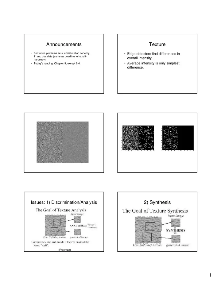
Announcements Texture • For future problems sets: email matlab code by • Edge detectors find differences in 11am, due date (same as deadline to hand in overall intensity. hardcopy). • Average intensity is only simplest • Today’s reading: Chapter 9, except 9.4. difference. 2) Synthesis Issues: 1) Discrimination/Analysis (Freeman) 1

Many more issues What is texture? 3. Texture boundary detection. • Something that repeats with variation. 4. Shape from texture. • Must separate what repeats and what stays the same. We’ll focus on 1, mention 2. • Model as repeated trials of a random process – The probability distribution stays the same. – But each trial is different. Texture Discrimination is then Simplest Texture Statistics • Each pixel independent, identically • Two sets of samples. distributed (iid ). • Do they come from the same random • Examples: process? – Region of constant intensity. – Gaussian noise pattern. – Speckled pattern Matlab How/why to compare Simplest Texture Discrimination • Compare histograms. • Simplest comparison is SSD, many others. • Can view probabilistically. – Divide intensities into discrete ranges. – Histogram is a set of samples from a probability – Count how many pixels in each range. distribution. – With many samples it approximates distribution. – Test probability samples drawn from same distribution. Ie ., is difference greater than expected when two samples come from same distribution? Matlab 0 - 25 26 - 50 51 - 75 76 - 100 225 - 250 2

Chi square distance between texton histograms More Complex Discrimination Chi - square • Histogram comparison is very limiting i – Every pixel is independent. } 0.1 – Everything happens at a tiny scale. j } Matlab k 0.8 • Use output of filters of different scales. − 2 K [ h ( m ) h ( m )] 1 ∑ χ = i j 2 ( h , h ) + i j 2 h ( m ) h ( m ) = m 1 i j ( Malik ) Example (Forsyth & Ponce) What are Right Filters? What are Right Filters? • Multi - scale is good, since we don’t know right • The more independent the better. scale a priori. – In an image, output of one filter should be • Easiest to compare with naïve Bayes : independent of others. Filter image one: (F1, F2, …) – Because our comparison assumes Filter image two: (G1, G2, …) independence. S means image one and two have same – Wavelets seem to be best. texture. Approximate: P(F1,G1,F2,G2, …| S ) By P( F1,G1|S)* P( F2,G2|S)*… 3

Spots and Oriented Bars Difference of Gaussian Filters ( Malik and Perona ) Gabor Filters Gabor filters at different scales and spatial frequencies Matlab top row shows anti-symmetric (or odd) filters, bottom row the symmetric (or even) filters. +   x y 2 2 + −   cos( k x k y ) exp σ   x y 2 2 4

Gabor filters are examples of Synthesis with this Representation (Bergen and Heeger) Wavelets • We know two bases for images: – Pixels are localized in space. – Fourier are localized in frequency. • Wavelets are a little of both. • Good for measuring frequency locally. Example 1 st Order Markov Model Markov Model • Captures local dependencies. • Each pixel is like neighbor to left + noise with some probability. – Each pixel depends on neighborhood. Matlab • Example, 1D first order model • These capture a much wider range of P(p1, p2, …pn ) = phenomena. P(p1)*P(p2|p1)*P(p3|p2,p1)*… = P(p1)*P(p2|p1)* P(p3|p2)*P(p4|p3)*… 5

There are dependencies in Filter Outputs • Edge – Filter responds at one scale, often does at other scales. – Filter responds at one orientation, often doesn’t at orthogonal orientation. • Synthesis using wavelets and Markov model for dependencies: – DeBonet and Viola – Portilla and Simoncelli We can do this without filters • Each pixel depends on neighbors. 1. As you synthesize, look at neighbors. 2. Look for similar neighborhood in sample texture. 3. Copy pixel from that neighborhood. 4. Continue. This is like copying, but not just repetition Photo Pattern Repeated 6

With Blocks Conclusions • Model texture as generated from random process. • Discriminate by seeing whether statistics of two processes seem the same. • Synthesize by generating image with same statistics. To Think About • 3D effects – Shape: Tiger’s appearance depends on its shape. – Lighting: Bark looks different with light angle • Given pictures of many chairs, can we generate a new chair? 7

This document was created with Win2PDF available at http://www.daneprairie.com. The unregistered version of Win2PDF is for evaluation or non-commercial use only.