SLIDE 1
Grafting Coordinates for Teichm¨ uller Space
October 2006
David Dumas (ddumas@math.brown.edu) http://www.math.brown.edu/˜ddumas/ (Joint work with Mike Wolf)
SLIDE 2
2
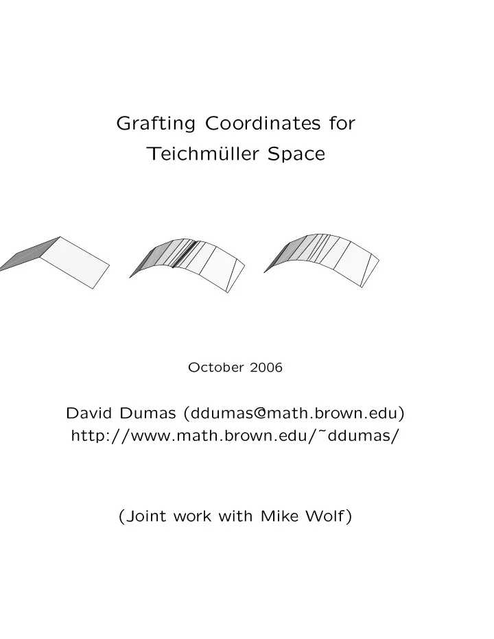
– Grafting – Start with X, a closed hyperbolic surface, and γ, a simple closed hyperbolic geodesic. Cut X along γ and insert a Euclidean cylinder of length t. The result is grtγ X, the grafting of X along tγ. Grafting extends continuously to limits of weighted geodesics, i.e. measured laminations. Intuitively, grafting replaces λ with a thickened version that has a Euclidean metric. [Thurston; Kamishima-Tan]
SLIDE 3 3
Thus grafting defines a continuous map gr : ML (S) × T (S) → T (S) where S is the smooth surface underlying X, T (S) is Teichm¨ uller space, ML (S) is the PL-manifold
Note dim T (S) = dim ML (S) = 6g − 6. Main Theorem For each X ∈ T (S), grafting X defines a homeomorphism gr• X : ML (S) → T (S) (i.e. λ → grλ X).
Actually, we show that this map is a tangentiable diffeo-
- morphism. Its (lack of) regularity is a key issue.
This is a natural complement to: Theorem (Scannell-Wolf) For each λ ∈ ML (S), the λ-grafting map grλ : T (S) → T (S) is a diffeomorphism. Our proof of the main theorem uses the Scannell- Wolf theorem and a complex-linearity technique of Bonahon.
SLIDE 4
4
– Proof Outline: Scannell-Wolf Thm –
Tanigawa: grλ : T (S) → T (S) is proper Thus it suffices to show that grλ is a local
diffeomorphism, for then grλ is a smooth covering map of a contractible space.
By the inverse function theorem, it suffices to
study the derivative of grλ.
Infinitesimal Sc-W theorem: The derivative
d grλ : TXT (S) → Tgrλ XT (S) is an injective linear map (⇒ isomorphism).
Proof of infinitesimal theorem is a PDE argu-
ment based on the prescribed curvature and geodesic equations, applied to the Thurston metric on grλ X (i.e. hyperbolic on X, Eu- clidean on the cylinder).
SLIDE 5 5
– Proof Outline: Main Theorem –
Tanigawa: gr• X : ML (S) → T (S) is proper As before, it then suffices to show that gr• X
is a local homeomorphism.
Bonahon: Grafting is tangentiable (≃ has one-
sided derivatives everywhere). So an infinitesi- mal analysis is possible, can reduce to:
Infinitesimal Main Thm If a (PL or tang’ble)
family λt
measured laminations satisfies
∂ ∂t
∂t
(The tangent map of gr• X has no kernel at λ0.)
Given a supposed counterexample (λt, X) to
the infinitesimal main thm, use shearing to create a family Xt ∈ T (S) such that i
∂
∂t
∂t
Thus ∂
∂t
- t=0+ Xt = 0. The way Xt is constructed
then gives ∂
∂t
This relationship between derivatives comes
from Bonahon’s theory of shear-bend cocycles and the complex duality between shearing and bending.
SLIDE 6 6
– Derivatives in ML (S) and Cocycles – Let λt be a PL family of laminations, t ∈ [0, ). (We use PL instead of tangentiable for simplicity.) Want to make sense of the derivative ˙ λ = ∂
∂t
(following Bonahon, Thurston). One way is to put λt in a train track chart. Then the derivatives of the edge weights at t = 0+ give a signed measure on the train track. Let Λ be the essential support of λt at t = 0, i.e. Λ = lim
t→0+ Λt
where Λt = supp(λt), using the Hausdorff topology on geodesic laminations. Typically Λ is bigger than the support of λ0.
SLIDE 7 7
The derivative ˙ λ can be interpreted as a transverse cocycle (finitely additive signed transverse mea- sure) for Λ. Can describe this cocycle using the train track derivative,
directly in terms
intersection numbers: i(˙ λ, τ) := lim
t→0+
i(λt, τ) − i(λ0, τ) t Assume Λ is maximal (complementary regions are ideal triangles) by enlarging it if necessary. Let H(Λ) be the vector space of transverse cocycles
H(Λ) ≃ R6g−6 So the family λt determines a vector ˙ λ ∈ H(Λ). Idea to construct Xt: Embed T (S) in H(Λ), then translate X by t˙ λ in this embedding to obtain Xt.
SLIDE 8 8
– Shearing – Given a maximal geodesic lamination Λ, Bonahon defines an embedding σ : T (S) → H(Λ), where σ(X) is the shearing cocycle of X: The lift of Λ to ˜ X ≃ H2 is a tiling by ideal triangles (not necessarily locally finite). The value of σ(X) on a transversal τ (lifted to
H2) connecting triangles TP and TQ is the relative
shear of TP and TQ. For example, if TP and TQ share an edge, then i(σ(X), τ) is the signed distance between the feet
- f the altitudes of TP and TQ on this edge.
Otherwise, identify the nearest edges of TP and TQ using “fans” of geodesics interpolating between the leaves of Λ separating TP and TQ.
SLIDE 9
9
Thm (Bonahon) The map σ : T (S) → H(Λ) is a real-analytic embedding; its image is an open convex cone with finitely many faces. Thus for all t sufficiently small, the sum σ(X) + t˙ λ is the shearing cocycle of some Xt ∈ T (S), and X0 = X. This is a shearing or cataclysm path. For example, if ˙ λ is supported on a singled closed geodesic γ, then Xt is obtained by twisting X along γ; if ˙ λ is a positive measure, then Xt is the associated earthquake path.
SLIDE 10 10
– Completing the proof – Finally, we use a remarkable complex linearity property of the derivative of grafting (with respect to the shearing embedding): Thm (Bonahon) Let Yt = grλt Xt where ˙ λ ∈ H(Λ) and ˙ σ = ∂
∂t
Then ˙ Y =
∂ ∂t
- t=0+ Yt is a C-linear function of the complex
cocycle (˙ σ + i˙ λ) ∈ H(Λ) ⊗ C. Recall that we started with (λt, X0) such that grλt X0 is constant to first order, and then used ˙ λ ∈ H(Λ) to construct a shearing path Xt. Applying the C-linearity theorem to (λ0, Xt) and (λt, X0) (with associated complex cocycles ˙ λ and i˙ λ, resp.) we find: i
∂
∂t
∂t
By Scannell-Wolf,
∂ ∂t
= 0, but in the shearing embedding ∂
∂t
λ. Thus ˙ λ = 0.
SLIDE 11 11
– Why C-linearity? – Thurston connected grafting with CP1 structures
The idea is to lift to the universal cover and exploit a natural equivalence: (Grafting ∆ ⊂ C ⊂ CP1) ↔ (Bending H2 ⊂ H3) This allows one to understand the derivative of grafting by studying the effect of a bending de- formation on the holonomy of a pleated surface (Bonahon; Epstein-Marden). The ultimate “source” of the complex linearity is: The hyperbolic isometry with translation s and twist t along a fixed axis is a holomorphic function
SLIDE 12 12
– Applications –
Comparing geometric and analytic perspectives
Every CP1 structure is obtained by projective grafting, giving CP1(S) ≃ ML (S) × T (S). Strata in CP1(S) with constant complex struc- ture project homeomorphically to both ML (S) and T (S) (by Scannell-Wolf and main thm, respectively).
Hyperbolic structure on convex hull boundary
parameterizes a Bers slice. Let M be a quasi-Fuchsian hyperbolic structure
- n S × R with ideal boundary Y ∪ Y ′ and convex
core boundary X ∪ X′. Then M is determined up to isometry by (X, Y ) ∈ T (S) × T (S).
SLIDE 13
13
– Applications –
Grafting coordinates, grafting rays.
For each X ∈ T (S), the map λ → grλ X gives “polar coordinates” for T (S) centered at X. Each ray in ML (S) maps to a grafting ray {grtλ X}t∈R+ in T (S), a properly embedded smooth path starting at X. Intuition: – For small t, the λ-ray is like i(twist), because the grafting cylinder is nearly geodesic. – For large t, it is like a Teichm¨ uller deforma- tion with horizontal foliation λ, because the grafting cylinder nearly fills S. Properties of the γ-ray (γ=simple closed geodesic): – Tangent vector at t = 0 is ∇WP(ℓγ) (Wolpert; McMullen). – Extremal length of γ is eventually monotone decreasing – Hyperbolic length of γ is eventually monotone decreasing