SLIDE 1 GAMBLING PREFERENCES, OPTIONS MARKETS, AND VOLATILITY
Benjamin M. Blaua, T. Boone Bowlesb, and Ryan J. Whitbyc Abstract: This study examines whether the gambling behavior of investors affect volume and volatility in financial markets. Focusing on the options market, we find that the ratio of call option volume relative to total option volume is greatest for stocks with return distributions that resemble lotteries. Consistent with theoretical predictions in Stein (1987), we demonstrate that gambling-motivated trading in the options market influences future spot price volatility. These results not only identify a link between lottery preferences in the stock market and the options market, but they also suggest that lottery preferences can lead to destabilized stock prices.
aBlau is an Associate Professor in the Huntsman School of Business at Utah State University,
Logan, Utah. Email: ben.blau@usu.edu. Phone: 435-797-2340.
bBowles is a Graduate Student in Financial Economics in the Huntsman School of Business at
Utah State University, Logan, Utah. Email: boone.bowles@gmail.com.
cWhitby is an Assistant Professor in the Huntsman School of Business at Utah State University,
Logan, Utah. Email: ryan.whitby@usu.edu. Phone: 435-797-9495.
SLIDE 2 1
I. INTRODUCTION Theoretical research has long studied the potential role of speculative trading and gambling preferences by investors.1 Markowitz (1952), for instance, suggests that some investors might prefer to purchase stocks that have a small probability of obtaining a large payoff. Barberis and Huang (2008) build on work by Kahneman and Tverksy (1979) and Benartzi and Thaler (1995) that examine the effect of prospect theory on asset prices. Barberis and Huang (2008) posit that some investors will overweight the tails in the return distribution and show preferences for positive
- skewness. They also demonstrate that skewness preferences can affect asset prices. Empirical
research tends to support the argument that (i) some investors prefer positive skewness (see Mitton and Vorkink (2007), Kumar (2009), and Kumar, Page, and Spatt (2011)) and (ii) investors’ preferences for positive skewness lead to price premiums and subsequent underperformance (Zhang (2005), Mitton and Vorkink (2007), Boyer, Mitton, and Vorkink (2010), Bali, Cakici, and Whitelaw (2011)). Both theoretical and empirical research supports the idea that some investors prefer skewness or lottery-type stock characteristics. In this study, we extend this literature in two ways. First, we examine whether stocks with characteristics that resemble lotteries have higher levels of call option volume. Second, and perhaps more importantly, we examine whether preferences for lotteries that are exhibited in higher call option volume influence future spot price volatility. While prior research indicates that informed trading might explain the motive to trade in the options market (Black (1975), Easley, O’Hara, and Srinivas (1998), and Pan and Poteshman (2006)),
- thers have suggested that speculative trading might also motivate investors to trade options (Stein
1 Examples include: Markowitz (1952), Arditti (1967), Simkowitz and Beedles (1978), Scott and Horvath (1980),
Conine and Tamarkin (1981), Stein (1987), Shefrin and Statman (2000), Statman (2002), Brunnermeier and Parker (2005), Brunnermeier, Gollier, and Parker (2007), and Barberis and Huang (2008).
SLIDE 3 2
(1987)). In this paper, we attempt to measure speculative trading in a variety of ways while focusing primarily on investors’ preferences for lottery-like returns (Golec and Tamarkin (1998) and Garrett and Sobel (1999)). Furthermore, because call options have limited downside risk and unlimited upside potential, these types of options might be an attractive security for investors with preferences for lotteries. Understanding the relation between preferences for lotteries and option markets is important given the findings of Pan and Poteshman (2006) and Johnson and So (2012), who show that option trading volume contains information about future returns in underlying stocks. We follow prior research and approximate lottery stocks in several ways. First, we proxy for lottery stocks by examining both positive total and positive idiosyncratic skewness in returns during the prior quarter (see Barberis and Huang (2008), Mitton and Vorkink (2007), Kumar, Page, and Spalt (2011), and Kumar and Page (2011)).2 Second, we follow Bali, Cakici, and Whitelaw (2011) and approximate lottery stocks as those with the largest maximum daily return. Third, following Kumar (2009) and Kumar and Page (2011), we approximate lottery stocks by calculating indicator variables that capture low-priced stocks that have the highest idiosyncratic volatility and the highest idiosyncratic skewness during the previous quarter. Using these approximations for lottery stocks, we then examine the fraction of total option volume that is made up from call
- ptions, which we denote as the call ratio for brevity. Observing a direct relation between call
ratios and these approximations of lottery stocks can provide an important contribute to literature that suggests that some investors have strong preferences for assets with lottery-like returns.
2 Following Kumar (2009), we also calculate systematic (or co-) skewness. However, since Kumar (2009) and
- thers generally use total and idiosyncratic skewness to measure lottery preferences, we focus most of tests on these
two measures of skewness instead of systematic skewness.
SLIDE 4 3
Our univariate results show a monotonically positive relation between call ratios and last- quarter’s total skewness. Similar results are found when examining the relation between call ratios and both last-quarter’s idiosyncratic skewness and last-quarter’s maximum daily return. When we approximate stock lotteries using low-priced stocks with the highest idiosyncratic volatility and the highest idiosyncratic skewness, we again show that call ratios are highest for these stocks. These results indicate that preferences for lottery-type stocks are reflected in a higher proportion
- f total option volume that is made up from call options.
We use a variety of multivariate tests to determine whether call ratios are higher for lottery
- stocks. After controlling for a variety of factors that influence the call ratio, we show a robust
positive relation between call ratios and our approximations for lottery stocks. These results support our univariate tests and indicate that investors’ penchant for lottery stocks, which has been identified in previous research (Zhang (2005), Mitton and Vorkink (2007), Kumar (2009), Boyer, Mitton, and Vorkink (2010), and Bali, Cakici, and Whitelaw (2011)), is also reflected in higher call ratios. Our second set of tests might have more important implications as we seek to explain whether call option investors with gambling preferences generate greater levels of volatility in underlying stock prices. In particular, we determine whether the relation between call ratios and lottery-like characteristics, as well as other speculative trading measures, affect the stability of underlying spot prices. These tests are motivated by theory in Stein (1987) which shows that speculative trading in derivatives markets can lead to more volatility in the spot market. The idea in Stein (1987) is that speculation can increase the level of noise trading, which adversely affects informed investors’ ability to stabilize prices. Our objective is to determine whether gambling and speculation in the options market leads to greater volatility in spot prices.
SLIDE 5 4
We first show that next-quarter’s volatility in spot prices is monotonically increasing across call ratios. We then decompose the call ratio into a speculative and a non-speculative component. The speculative component of the call ratio contains the portion of the call ratio that is related to lottery-like characteristics and other speculative trading measures. The non-speculative component of the call ratio is the portion of the call ratio that is orthogonal to these characteristics. For brevity, we refer to the portions of the decomposed call ratio as the speculative call ratio and the non-speculative call ratio, respectively. We show that next-quarter’s idiosyncratic volatility is directly related to the speculative call ratio. However, next-quarter’s idiosyncratic volatility is unrelated to the non-speculative call ratio. Our multivariate tests show that, after controlling for other factors that influence next- quarter’s volatility, the relation between the total call ratio and future volatility is only marginally
- significant. However, the speculative call ratio is directly related to next-quarter’s idiosyncratic
volatility and the relation is both statistically significant and economically meaningful. When including the same controls, we do not find a significant relation between next-quarter’s idiosyncratic volatility and the non-speculative portion of the call ratio. These results indicate that speculative call option activity adversely affects the stability of underlying stock prices while non- speculative call option activity does not. Our study contributes to the literature in two important ways. First, our finding that call ratios are directly related to stock characteristics that resemble lottery-like features supports the growing line of research that suggests that some investors have strong preferences for lottery stocks (Zhang (2005), Mitton and Vorkink (2007), Barberis and Huang (2008), Kumar (2009), Boyer, Mitton, and Vorkink (2010), Bali, Cakici, and Whitelaw (2011), Kumar, Page, and Spalt (2011), and Kumar and Page (2011)). Second, our results that identify a link between future spot
SLIDE 6
5
price volatility and speculative call ratios are consistent with theory in Stein (1987), which posits that speculative trading activity in the derivatives market can lead to increased volatility in the spot market. II. RELATED LITERATURE AND HYPOTHESIS DEVELOPMENT Barberis and Huang (2008) show that investors tend to overweight the tails of return distributions, which leads to observed preferences for positive skewness. Skewness preferences can result in an equilibrium that leads to overpriced, positively skewed stocks. Price premiums that are caused by skewness preferences will underperform stocks that are not positively skewed. Empirical research tends to support the predictions in Barberis and Huang (2008). For instance, Mitton and Vorkink (2007) find that some investors sacrifice mean-variance efficiency in their portfolios by underdiversifying. Further, portfolios that are underdiversified exhibit more positive skewness than portfolios that are well diversified. Both Zhang (2005) and Boyer, Mitton, and Vorkink (2010) show that stocks with positive skewness underperform stocks with negative skewness, which is consistent with the idea that skewness preferences lead to price premiums and subsequent underperformance. In a related study, Kumar (2009) approximates lottery-type stocks as those stocks with the lowest prices, the highest idiosyncratic volatility, and the highest idiosyncratic skewness. Kumar (2009) finds that individual investors have greater preferences for lottery-type stock characteristics than do institutional investors. Further, Kumar (2009) shows that investors with preferences for lottery stocks have similar socioeconomic characteristics to those individuals that participate in state lotteries. These results support the idea that some investors have preferences for stocks with lottery-like payoffs. Using a variety of different empirical tests, Kumar (2009) shows that lottery stocks significantly underperform non-lottery stocks thus supporting the predictions in Barberis
SLIDE 7 6
and Huang (2008). Similar conclusions are drawn in Bali, Cakici, and Whitelaw (2011), who show that stocks with the largest maximum daily return underperform other stocks. Again, these results support the idea that stocks with a low probability of an extreme payoff exhibit price premiums and subsequent underperformance. Stein (1987) posits that the availability of financial derivatives, such as options and futures, provides investors with a natural way to speculate about spot price movements. For instance, a call option allows the buyer the opportunity to limit the down-side risk while having unlimited up- side potential. It is natural, therefore, to suggest that call options provide investors the opportunity to trade on their preferences for positive skewness or other lottery-like features. Our first hypothesis indirectly examines the conjecture made by Stein (1987) that derivative markets augment speculative trading in the spot market. The first null hypothesis is stated below: H1: Call ratios are unrelated to features that resemble lottery-type stock characteristics. The null hypothesis H1 suggests that the call ratio is unrelated to past total skewness, past idiosyncratic skewness, stocks with the largest maximum daily return, or stocks that have the lowest prices, the highest idiosyncratic volatility, and the highest idiosyncratic skewness. If call
- ptions are an important avenue for speculative gambling based on characteristics of the return
distributions of the underlying asset, then we will reject the null hypothesis H1 if call ratios are directly related to lottery-like features.3 In a recent study that is related to our first hypothesis, Boyer and Vorkink (2013) investigate the relation between total skewness and returns on equity options. They find that total
3 We recognize an important limitation in our study. We are unable to determine the initiators of the call volume
used in this study. While prior research has obtained signed option volume from proprietary sources, we do not have access to this type of data. However, other studies have used total call volume ratios instead of signed call
- ption volume to determine the effect of call volume on asset prices. For instance, Johnson and So (2012) examine
the relation between call-to-put ratios and future skewness.
SLIDE 8 7
skewness is negatively related to average option returns. Given the inherent speculative properties in options, they conclude that investor demand for lottery-like options results in larger option premiums that could be compensation for non-hedgable risk encountered by intermediaries that make markets in options. While they focus entirely on the distribution of option returns, our tests are different as we focus on option trading activity and the distribution of underlying stock returns. Our tests, however, are complementary in that both studies examine the impact that preferences for lottery-like securities can have on the intertemporal dynamics of traded assets. Gambling in the options market may or may not have an effect on the stability of prices in the spot market. A theoretical debate about whether speculation stabilizes or destabilizes asset prices has been contested in the literature. Ross (1976) uses Arrow’s (1964) state space approach and argues that the availability of options can improve the efficiency of markets by opening new spanning opportunities. While there may be a finite number of stocks an investor can buy, there are virtually an infinite number of combinations of options an investor can buy. Ross (1976) therefore argues that increasing the number of opportunities to trade can lead to greater market
- efficiency. Friedman (1953), Danthine (1978), and Turnovsky (1983) also argue that speculative
behavior can provide a stabilizing influence to prices. On the other hand, Salant (1984) and Hart and Kreps (1986) show that in general equilibrium, speculation can lead to price destabilization. Stein (1987) presents a model that allows for speculation in derivatives markets and partitions the effect of speculation into two categories. Stein’s (1987) two-period model allows for both spot market traders and secondary (i.e. derivatives) market traders. Under various scenarios, the increase of speculators in the derivatives market actually stabilizes prices. When derivative traders are perfectly or completely uninformed, speculation results in more stable prices because there are no informational externalities present to
SLIDE 9 8
- ffset the risk sharing benefits associated with increased trading in the derivatives market.
However, for cases when derivative traders have less-than-perfect information, an increase in speculation results in more volatile spot prices. Specifically, when derivative traders have intermediate levels of information, their actions are unpredictable and risk-averse spot traders back away from the market, which leads to destabilized prices. In general, the imperfect information environment can create uncertainty that can result in greater spot price volatility. The model in Stein (1987) does not rely on any irrationality or behavioral assumption, but rather on imperfect information held by speculators. This assumption does not seem overly restrictive, given our setting in the stock and options markets. In fact, assuming that options traders have perfect or zero information seems much less likely. Stein (1987) therefore contends that the availability of options provides a greater level of risk sharing among investors which can improve social welfare by stabilizing spot prices. However, in an imperfect information environment, greater levels of speculation in derivatives markets can produce noisy prices which adversely affect the ability of informed investors to transmit information into prices, thus leading to more volatility. Speculation in the options market can become destabilizing when the effect of less information transmission due to noisy prices
- utweighs the effect of greater risk sharing. If this condition holds, then our second null hypothesis
follows: H2: Speculative call ratios will have a similar effect on future spot price volatility as non- speculative call ratios. The null hypothesis H2 suggests that the speculative portion of the call ratio will have the same effect on future spot price volatility as the non-speculative portion of the call ratio. If speculative
- ption trading destabilizes spot prices, then we can reject H2 by showing that speculative call
SLIDE 10 9
- ption activity directly affects future spot price volatility more than non-speculative call option
- activity. We test these two hypotheses below.
III. DATA DESCRIPTION The data used in this study is obtained from several different sources. From the Center for Research on Security Prices (CRSP), we gather daily and monthly stock prices, volume, returns, and market capitalization. From Bloomberg, we gather daily call option volume and put option volume.4 From Compustat, we obtain quarterly financial statement information such as total assets and total liabilities. We also obtain institutional holdings from 13f filings. After merging the Compustat data to the available stocks from our other data sources, we are left with 3,112 stocks and 61,689 stock-quarter observations. Our sample time period is 1997 to 2007. We aggregate stock trading volume and option volume to the quarterly level for each stock. We also obtain the closing price and the market capitalization on the last day of each quarter. Table 1 reports statistics that summarize the data. The table shows that the average stock has a quarterly market capitalization (Size) of nearly $6.8 billion and a price (Price) of $29.68. Using institutional holdings, we estimate the fraction of shares outstanding that are held by institutions (InstOwn). The average stock has InstOwn of 0.6677, a book-to-market ratio (B/M) of 0.2029, and a debt-to-assets ratio (D/A) of 0.5075. Using quarterly stock trading volume, we calculate the share turnover (Turn), or the portion of shares outstanding that are traded during a particular quarter. The mean turnover is 6.37. We calculate idiosyncratic volatility (IdioVolt) by taking the standard deviation of residual returns from a daily Fama-French Four-Factor model during each quarter. The average stock has an IdioVolt of 0.0256.
4 The daily option volume obtained from Bloomberg is the total volume for options at all strike prices for all
expirations.
SLIDE 11 10
Table 1 also reports stock characteristics that resemble lotteries. To obtain estimates of these characteristics, we use daily returns and estimate total skewness by taking the third moment using the following formula. − − − =
∑
= 3 1 3
ˆ ) ( ) 2 )( 1 ( σ
n t t
r r n n n TotSkew (1) rt is the CRSP raw return for a particular stock on day t, r is the mean return for a particular stock during a particular quarter, and σ ˆ is the estimate for the standard deviation of returns for the stock during the quarter. We also calculate idiosyncratic skewness and systematic skewness (or co- skewness) following Kumar (2009). In particular, we estimate idiosyncratic skewness (IdioSkew) by first fitting a daily two-factor model where the factors are the market risk premium and the market risk premium squared. We then estimate equation (1) using residual returns from this two- factor model instead of using CRSP raw returns. From the two-factor model, systematic skewness (SystSkew) is the coefficient on the market risk premium squared. We note that the literature that discusses preferences for lottery-type stocks generally uses total skewness or idiosyncratic skewness instead of systematic skewness. However, we include systematic skewness in some of
- ur initial tests following Kumar (2009). These measures of skewness are estimated in each
quarter from 1997 to 2007.5 The motivation to use skewness to approximate lotteries is based on theory in Barberis and Huang (2008). Lotteries exhibit positively skewed return distributions, where a large majority of the distribution is at values less than the mean and a small portion of the
5 We use the quarterly frequency based on arguments in Xu (2007) that suggest that when estimating higher
moments, like return skewness, more observations are required. Xu (2007) requires 40 days of returns to estimate return skewness. We therefore estimate skewness at the quarterly level thus allowing for a greater number of
- bservations when calculating higher moments.
SLIDE 12 11
distribution is in the long tail that is greater than the mean. The average stock has TotSkew of 0.2331, IdioSkew of 0.2478, and SystSkew of -0.2062. As an additional proxy for lottery-type characteristics, we follow Bali, Cakici, and Whitelaw (2011) and estimate the maximum daily return during a particular quarter for each stock in our sample (MaxRet). Table 1 reports that the mean MaxRet is 0.0938. In addition to examining these low probability-high payoff events, we also follow Kumar (2009) and construct two indicator variables: LOTTERY1 and LOTTERY2. We sort stock-quarter observations into quartiles based on last quarter’s stock price, last quarter’s idiosyncratic volatility, and last quarter’s idiosyncratic
- skewness. If a particular stock has (i) a price that is less than the median, (ii) idiosyncratic volatility
greater than the median, and (iii) idiosyncratic skewness that is also greater than the median, then LOTTERY1 is equal to one and zero otherwise. Additionally, LOTTERY2 is equal to one if a particular stock has (i) a price that in the lowest price quartile, (ii) idiosyncratic volatility in the highest idiosyncratic volatility quartile, and (iii) idiosyncratic skewness in the highest idiosyncratic skewness quartile.6 The average stock has a value for LOTTERY1 of 0.1926 and a value of LOTTERY2 of 0.0510. We note that the when we calculate these indicator variables, we re-sort stock-quarter observations into quartiles during each quarter. Table 1 also reports summary statistics for option activity. CallVol is the number of call
- ptions contracts traded during a particular quarter while PutVol is the number of put option
contracts trading during the same quarter. The average stock has CallVol (PutVol) of 65,041 (39,397) during a particular quarter. The main variable of interest in this study is the call ratio. We calculate the call ratio (CR) as the fraction of total option volume that is made up from call
- ptions. The average stock has a CR of 0.6726.
6 For a more extensive discussion on these last two approximations of lotteries, see Kumar (2009), pp. 1896.
SLIDE 13 12
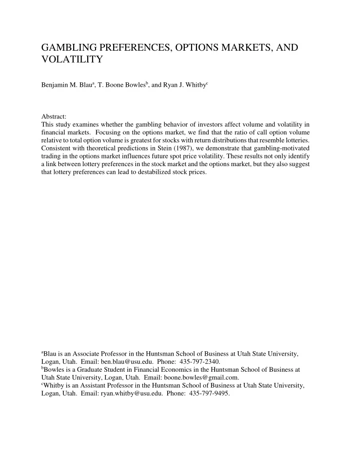
Figure 1 also provides an important description of the data used throughout the analysis. The figure reports the time series percentages of (i) the universe of stocks that are considered lottery-type stocks according to Kumar (2009), (ii) stocks that have tradable options, and (iii) lottery-type stocks that have tradable options. The percent of the universe of stocks available on CRSP that are considered lottery stocks (LOTTERY1 = 1) remained relatively close to 20% during
- ur sample time period.7 On the other hand, the percent of stocks that have tradable options has
increased from less than 20% to nearly 43% during our sample. Similarly, the percent of lottery- type stocks that have tradable options began at approximately 7% and has increased to more than 27%. IV. EMPIRICAL RESULTS In this section, we first test H1 by examining the relationship between option trading activity and our approximations for stock lotteries. Second, we test H2 by determining whether the speculative and non-speculative portion of call option trading activity affects next-quarter’s spot price volatility. IV.A. The Relation Between Call Ratios and Stock Lotteries – Univariate Tests We begin our tests of H1 by sorting stock-quarter observations into quartiles based on the lottery-type stock characteristics discussed in the previous section. We then report call ratios across quartiles. Table 2 reports the results of the analysis. Panel A shows the results when we sort by the continuous proxies for lottery stocks while Panel B presents the findings when we sort based on the indicator variables LOTTERY1 and LOTTERY2. We re-sort stock-quarter
7 It might also be noteworthy to discuss some of the stock characteristics that are related to the variable LOTTERY1.
In unreported tests, we estimate the correlation between LOTTERY1 and some of the other variables discussed in Table 1. We find that LOTTERY1 is inversely related to market cap, share price, institutional ownership, and the debt-to-asset ratio. We also find that LOTTERY1 is directly related to book-to-market ratios, share turnover, and (by construction) idiosyncratic volatility and idiosyncratic skewness.
SLIDE 14 13
- bservations at the beginning on each quarter. In Panel A column [1], we see that call ratios are
increasing monotonically across increasing TotSkewi,t-1 quartiles. Column [1] reports that the difference between extreme quartiles (QIV – QI) is 0.0297 (p-value = <.0001). We also estimate correlation coefficients between CR and TotSkewt-1 and find that call ratios are directly related to TotSkewi,t-1 (correlation = 0.0557, p-values = <.0001). These results indicate that the fraction of total option volume that is made up of call options depends on the level of total skewness of the spot asset during the previous quarter. Column [2] reports the results when sorting by last quarter’s idiosyncratic skewness. Similar to our findings in Panel A, we find that call ratios are increasing monotonically across last quarter’s idiosyncratic skewness. Further, we show that call ratios are highest in stocks with the highest idiosyncratic skewness. In column [3], we do not find that call ratios are monotonically increasing across quartiles sorted by systematic skewness. In fact, we find that call ratios are generally decreasing. These results are somewhat expected given the findings in Kumar (2009) that show that investors (and in particular, individual investors) have lower preferences for stocks with systematic skewness. Further, other studies (Mitton and Vorkink, 2007; Kumar, 2009; Boyer, Mitton, and Vorkink, 2010; Kumar, Page, and Spalt; 2011; Kumar and Page, 2013) focus on idiosyncratic skewness when identifying preferences for lottery-type stocks. Therefore, systematic skewness might not be the best proxy for gambling preferences and tests of H1. Column [4] shows the results when we sort stocks into quartiles based on the prior quarter’s maximum daily stock
- return. Consistent with our findings in columns [1] and [2], we show that call ratios are
monotonically increasing across increasing quartiles. Further, the difference between extreme quartiles is positive and significant and the correlation is also economically meaningful. Results in columns [1], [2], and [4] seem to reject the null hypothesis H1 and suggest that call ratios are
SLIDE 15 14
directly related to past skewness and indicate that preferences for skewness are reflected in higher call ratios. Next, we test H1 by examining the relation between call ratios and the two indicator variables that are used to approximate stock lotteries. We partition our sample of stock-quarter
- bservations into two subsamples based on the indicator variables. Focusing first on column [1],
we find that the mean call ratio for stock-quarter observations when LOTTERY1 = 1 is 0.7275. Mean call ratios in the subsample LOTTERY1 = 0 is 0.6595. The difference in means is -0.0680 and is statistically significant (p-value = <.0001). In economic terms, this difference is more than ten percent of the call ratio in stocks where LOTTERY1 = 0. We also find that the correlation is 0.1552 (p-value = <.0001) suggesting that the call ratios are markedly higher in stocks that resemble lotteries. In column [2], the mean call ratio is also statistically and economically larger in the subsample of stocks where LOTTERY2 = 1. The difference between classifications is - 0.0909 (p-value = <.0001). This difference is nearly 14 percent of the call ratio for stocks where LOTTERY2 = 0. Results in Panel B further support our findings in Panel A and reject the null hypothesis H1. These univariate tests seem to suggest that call ratios are directly related to spot- asset characteristics that approximate lotteries. Further, our findings are stronger in economic magnitude when we identify stock lotteries using the definition in Kumar (2009), Kumar, Page, and Spalt (2011), and Kumar and Page (2013). IV.B. The Relation Between Call Ratios and Stock Lotteries – Multivariate Tests In the previous section, our univariate tests reject H1 and show a positive relation between call ratios and stock lotteries. We recognize the need to control for other factors that might influence the level of call ratios. Therefore, we estimate the following equation using pooled data.
SLIDE 16 15
Call Ratioi,t = α + β1ln(sizei,t) + β2ln(pricei,t) + β3InstOwni,t + β4B/Mi,t + β5D/Ai,t + β6Turni,t + β7IdioVolti,t + β8Returni,t + β9Lottery-Characteristicsi,t-1 + εi,t (2) The dependent variable is the call ratio for stock i in quarter t (Call Ratioi,t). The independent variables include the natural log of market capitalization (ln(sizei,t)), the natural log of the stock price (ln(pricei,t)), institutional ownership (InstOwni,t), the book-to-market ratio (B/Mi,t), the debt- to-assets ratio (D/Ai,t), the quarterly share turnover (Turni,t), idiosyncratic volatility (IdioVolti,t), and the quarterly return (Returni,t). The independent variables of interest are the six Lottery- Characteristics described above. We note that a Hausman Test rejects the presence of random effects while an F-test finds observed differences across both stocks and days. Therefore, we estimate equation (2) while controlling for both stock and quarter fixed effects.8 The estimate for β9 determines whether we reject or fail to reject the null hypothesis H1. Table 3 reports the two-way fixed effects estimates. It is possible that our results might be biased due to multicollinearity. We handle this possibility in two ways. First, we estimate variance inflation factors and find that these factors that estimate the magnitude of inflation in standard errors caused by multicollinearity are all below three. These unreported tests indicate that our results are not subject to an abnormal amount of multicollinearity bias. Second, we estimate variants of equation (2) by including different combinations of control variables. Although the results from these tests are not reported, our findings are qualitatively similar to those reported in Table 3. Column [1] reports the results when TotSkewi,t-1 is the variable of interest. We find that market capitalization and quarterly returns are directly related to call ratios while share prices, institutional ownership, share turnover, and idiosyncratic volatility are inversely related to call
8 We note that qualitatively similar results are found when we use pooled OLS regressions and control for
conditional heteroskedasticity using White (1980) robust standard errors.
SLIDE 17 16
- ratios. Consistent with our univariate tests in the previous table, we find that the estimate for
TotSkewi,t-1 is positive and significant (estimate = 0.0062, p-value = <.0001). In economic terms, for every one standard deviation increase in total skewness, call ratios increase approximately 75 basis points. Column [2] shows that when including IdioSkewi,t-1 as the variable of interest, the coefficient is similar in sign and magnitude. In column [3], we do not find that SystSkewi,t-1 produces a coefficient that is reliably different from zero. This result is interesting in light of our findings in Table 2, which show a negative relation between call ratios and systematic skewness. Column [3] suggests that after controlling for other factors that might influence the call ratio, the systematic skewness of returns in the previous quarter is unrelated to call ratios. Again, this result is not surprising as the literature discussing preferences for lottery-type stocks uses total skewness
- r idiosyncratic skewness to proxy for lottery characteristics.
Column [4] reports the results when including MaxReti,t-1 as the variable of interest. Consistent with our findings in Table 2, MaxReti,t-1 produces a positive and significant estimate (estimate = 0.0457, p-value = <.0001). In economic terms, a one standard deviation increase in the prior quarter’s maximum daily return increases call ratios nearly 40 basis points. Columns [5] and [6] present the results when including LOTTERY1 and LOTTERY2 as the independent variables of interest. Consistent with our univariate tests in Table 2, we find that both LOTTERY1 and LOTTERY2 produce coefficients that are reliably different from zero (estimates = 0.0149, 0.0118; p-values = 0.000, <.0001). Combined with our tests in the previous table, these results again suggest that call ratios are higher for stocks that represent lotteries and reject the null hypothesis H1. IV.C. The Effect of Lottery Preferences on Spot Price Volatility – Univariate Tests
SLIDE 18
17
In this subsection, we test our second hypothesis H2, which suggests that the speculative portion of the call ratio will have a similar affect on spot price volatility as the non-speculative portion of the call ratio. Stein (1987) shows that, under certain conditions, speculation in derivatives markets can destabilize prices. We attempt to empirically test this conjecture by examining the relationship between next-quarter’s volatility and this quarter’s speculative/non- speculative call ratios. While we are interested in isolating the effect of gambling preferences in the options market on future spot price volatility as part of our tests of H2, we recognize the need to provide a broader definition of speculative trading. Few studies have tested Stein’s theory because of the difficulty in determining which trades are speculative in nature and which trades are not. In this section and those that follow, we attempt to decompose the call ratio into speculative and non-speculative portions. Before doing so, we note that while the theoretical literature is robust when discussing speculative trading, very few empirical studies have provided estimates for speculative trading activity. In order to obtain the speculative portion of the call ratio, we must first measure the amount of speculative sentiment in a particular stock. We do so in three ways. The first way we approximate speculative sentiment in a particular stock is by accounting for investors’ preferences for lottery stocks that are reflected in higher call ratios. Golec and Tarmakin (1998) and Garrett and Sobel (1999) suggest that preferences for skewness represent gambling or speculative preferences. Given the literature that discusses some investors’ preferences for lottery stocks, it is possible that these preferences, which might distort the traditional mean-variance preferences assumed by asset pricing theory, can create noisy prices thus leading to higher levels of volatility in the spot market (Stein, 1987). Therefore, when decomposing the call ratio into speculative and non-speculative portions, we first account for the
SLIDE 19 18
relation between call ratios and lottery-type stock characteristics that have been discussed in the previous section. As a second measure of speculative sentiment in a particular stock, we follow Llorente, Michaely, Saar, and Wang (2002), who develop a theoretical model that examines the dynamic relation between trading volume and stock returns, to approximate speculative trading.9 Their theory suggests that hedging trade volume will generate negatively autocorrelated returns while speculative trade volume will generate positively autocorrelated returns. Since Lo and Wang (2000) show that the daily time series of stock turnover is nonstationary, Llorente et al. (2002) de- trend the time series of the log of daily share turnover. We also follow prior research (Campbell, Grossman, and Wang, 1993; Llorente et al., 2002; and Covrig and Ng, 2004) and add a small constant (0.00000255) to turnover to account for days without trading volume. This constant is further shown to normalize the distribution of trading volume in Llorente et al. (2002) and Covrig and Ng (2004). Daily turnover is estimated in the following way for stock i on day t. log turni,t = log(turni,t + 0.00000255) (3) vi,t =
∑
− =
−
1 200 , ,
log 200 1 log
s t i t i
turn turn (4) vi,t is the de-trended measure of trading activity and is obtained by taking the difference between the log of turnover and mean of the log of turnover from day t-1 through t-200, where day t is the
9 In a recent study by Han and Kumar (2013), they find that stocks with a high proportion of retail trading exhibit
lottery-like features and suggests that “retail trading proportion” (RTP) can proxy for speculative trading. RTP is
- btained by calculating the ratio of dollar volume from small trades (less than $5,000 in dollar volume) to total stock
trading dollar volume during a particular time period. Because of order splitting by institutional traders after the decimalization period in 2001, Han and Kumar (2013) suggest that RTP might not capture retail trading and therefore they truncate their sample at 2000. In unreported tests that use proxies for speculative trading, we calculate RTP for the first part of our sample time period (1997 to 2000) and conduct some robustness tests. In general, we are able to draw similar conclusions whether we use Llorente et al.’s (2002) measure of speculative trading or RTP as in Han and Kumar (2013).
SLIDE 20 19
current trading day. We follow the empirical methods of Llorente et al. (2002) and approximate speculative trading by estimating the following time series equation for each stock in our sample. Reti,t+1 = β0 + β1Reti,t + β2Reti,t×vi,t+ εi,t+1 (5) The equation above provides a simple autoregressive formula where daily returns for each stock
- n day t+1 are regressed on daily returns for each stock on day t. According to Llorente et al.
(2002), the interaction between Reti,t and vi,t in equation (5) produces the estimate for speculative
- trading. The idea is that the larger (and more positive) the estimate for β2, the more likely that
trading activity increases the return autocorrelation. To the extent that speculative trades will generate greater return autocorrelation, the estimate for β2 proxies for speculative trading. Llorente et al. (2002) argue that a positive coefficient for β2 represents the degree of speculative trading in a particular stock while a negative coefficient for β2 provides an estimate for hedging
- activity. We estimate equation (5) and obtain the coefficient β2, which, for brevity, we denote as
Spec hereafter. The mean for Spec in our sample is very close to zero (mean = -0.0056) and seems to be normally distributed. Since Llorente et al. (2002) argue that it is positive estimates of β2 that represent speculative trading in a particular stock, we create an indicator variable SPEC_DUMMY that equals one if a stock has an estimate of β2 in the highest quartile. Stocks with SPEC_DUMMY equal to one have the most positive estimates of β2 and therefore, have the most speculative trading according to the arguments in Llorente et al. (2002). Speculative call ratios might lead to higher volatility in underlying security prices because of the argument in Stein (1987). When attempting to obtain the speculative portion of the call ratio, we will account for the relation between call ratios and this measure of speculative trading. The third and final way we measure speculative sentiment is by including a measure of market-wide, investor sentiment. Baker and Wurgler (2007) construct an investor sentiment index
SLIDE 21 20
using principle components analysis on six variables that might influence the sentiment of investors, which we denote as BW_Sentiment for brevity.10 We recognize that investor sentiment does not represent speculative sentiment, per se. However, we argue that the two types of sentiment are related and, when decomposing the call ratio, it will be important to account for the relation between the call ratio and the sentiment index. The correlation coefficient for call ratios and BW_Sentiment is 0.0184 (p-value = <.0001). While investors may use call options for a variety
- f reasons (information, speculation, hedging, etc.), in our decomposition of the call ratio, we are
interested in capturing the portion of the call ratio that is related to speculative trading and the portion that is unrelated to speculative trading. With our three measures of speculative sentiment, we decompose the call ratio in the following way. First, we estimate the following four regressions. Call Ratioi,t = α + β1 LOTTERY1 + β2SPEC_DUMMYi,t+ εi,t (6) Call Ratioi,t = α + β1 LOTTERY1 + β2MaxReti,t-1 + β3SPEC_DUMMYi,t+ εi,t (7) Call Ratioi,t = α + β1 LOTTERY1 + β2MaxReti,t-1 + β3IdioSkewi,t-1 +β4SPEC_DUMMYi,t+ εi,t (8) Call Ratioi,t = α + β1 LOTTERY1 + β2MaxReti,t-1 + β3IdioSkewi,t-1 +β4SPEC_DUMMYi,t+ β5BW_Sentimenti,t+ εi,t (9) We estimate each of these equations for each stock and obtain the predicted values and the
- residuals. To the extent that the variables included in the specifications properly represent
speculative sentiment, the predicted values can be interpreted as the speculative portion of the call ratio. The residuals, on the other hand, contain the portion of the call ratio that is orthogonal to the measures of speculative sentiment and therefore, represent the non-speculative call ratio.11
10 The six components are trading volume on the NYSE, the dividend premium, the closed-end fund discount, the
number and first-day returns on IPOs, and the share price of new equity issues.
11 It is possible to refer to the residuals from the estimated regressions as the hedging portion of the call ratio,
however, we are cautious of doing so given the difficultly of identifying speculative sentiment versus hedging
SLIDE 22 21
We denote
(1)i,t and ε(1) as the speculative call ratio and the non-speculative call ratio for our
first specification from equation (6). Likewise, we denote
(2)i,t and ε(2) as the speculative call
ratio and the non-speculative call ratio for our second specification from equation (7). Similarly,
(4)i,t, and ε(4) are defined using our third and fourth specifications (equations 8 and
9), respectively. We recognize the need to highlight the slight differences between equations (6) through (9). While we include LOTTERY1 and SPEC_DUMMY in each of the regressions, we also add the previous quarter’s maximum daily return in equation (7), the idiosyncratic skewness of the previous quarter’s returns in equation (8), and the Baker and Wurgler (2007) investor sentiment index in equation (9). Our objective in reporting the results from these four different specifications is to provide some robustness. We further note that in unreported tests, we include LOTTERY2 instead of LOTTERY1 in each specification and find the results to be similar to those reported in this study. Further, we also use total skewness instead of idiosyncratic skewness and find similar results. In addition, we estimate regressions that include various combinations of the measures used in equation (9) and are able to draw similar conclusions.12 Table 4 reports summary statistics for the predicted values and residuals obtained from estimating equations (6) through (9). The mean predicted values range from 0.6721 to 0.6726. By construction, the mean of each of the residuals is zero. The table also shows that the medians for
- sentiment. As discussed above, few empirical studies have provided approximations for speculative trading. Even
fewer have provided proxies for hedging activity. Therefore, we use the term non-speculative call ratios instead of hedging call ratios recognizing that we do not directly attempt to identify the hedging portion of the call ratio.
12 In addition to the variety of specifications, we have also estimated simple regressions where the dependent
variable is the call ratio and the single independent variable is each of the proxies for lottery stocks. We then take the predicted value of these simple regressions to approximate the speculative call ratio and the residuals to approximate the non-speculative call ratios. We are able to draw conclusions from these unreported tests that are similar to the conclusions drawn in this study.
SLIDE 23
22
both the predicted values and the residuals are close to the means. A closer examination of the table shows that both the predicted values and the residuals are distributed normally. With our approximations for speculative and non-speculative call ratios, we are ready to provide univariate tests of the null hypothesis H2, which suggests that the effect of speculative and non-speculative call ratios on future spot price volatility will be similar. We begin by first sorting the data into quartiles based first on the dependent variable in equations (6) through (9), which we denote for exposition as the total call ratio. This total call ratio contains both the portion of the ratio that is orthogonal to our measures of speculative sentiment (non-speculative call ratio) and the portion of the ratio that is directly related to our measures of speculative sentiment (speculative call ratio). After sorting the data based on the total call ratio, we then report next-quarter’s idiosyncratic volatility in the underlying stock across total call ratio quartiles. Column [1] of Table 5 presents these results. In column [1], we find that next-quarter’s idiosyncratic volatility is increasing monotonically across total call ratio quartiles. The column also reports the difference between extreme quartiles (difference = 0.0041, p-value = <.0001) as well as the univariate correlation coefficient (correlation = 0.1318, p-value = <.0001). These results suggest that call ratios are directly related to next-quarter’s idiosyncratic volatility and indicate that higher call ratios destabilize stock prices. Columns [2] through [5] present the results when sorting stocks into quartiles based on the predicted values from equations (6) through (9). The results in these columns indicate that next-quarter’s spot price volatility is monotonically increasing across speculative call ratios. We note that this positive relation is robust to each of the predicted values from the four specifications. We further note that the differences between extreme quartiles in columns [2] through [5] are 68% to 105% larger than the difference between extreme quartiles in column [1]. Further, the correlation coefficients in columns [2] through [5] are larger in magnitude
SLIDE 24
23
than the correlation coefficient in column [1]. These results seem to indicate that the direct relation between total call ratios and next-quarter’s idiosyncratic volatility is driven by the portion of the call ratio that is related to speculative sentiment. Columns [6] through [9] present the results when we sort by the estimated residuals from equations (6) through (9). Interestingly, when we sort stocks into quartiles based on our approximations for non-speculative call ratios, we find that next-quarter’s volatility is neither increasing nor decreasing. The differences between extreme quartiles are negative instead of positive as in earlier columns. Further, the correlation coefficients are not statistically significant in columns [7] and [8]. Combined with our findings in column [1] through [5], these results suggest that the portion of the call ratio that is unrelated to our measures of speculative sentiment has little, if any, impact on future idiosyncratic volatility. We are thus able to reject the null hypothesis H2 and conclude that while non-speculative call ratios are unrelated to future idiosyncratic volatility, speculative call ratios indeed affect the future idiosyncratic volatility in the spot market. IV.D. The Effect of Lottery Preferences on Spot Price Volatility – Multivariate Tests In this section we provide multivariate tests of the null hypothesis H2. We begin by estimating the following equation using pooled data. Ln(IdioVolti,t+1) = α + β1ln(Sizei,t+1) + β2ln(Pricei,t+1) + β3ln(IdioVolti,t) + β4ln(1+InstOwni,t+1)+ β5B/Mi,t+1 + β6D/Ai,t+1 + β7Returni,t + β8IdioSkewi,t+1 + β9FirmAgei,t+1 + β10Turni,t+1 + β11VariousCallRatios,t+ εi,t+1 (10) Equation (10) closely follows the specification of Brandt, Brav, Graham, and Kumar (2010). For example, the dependent variable is the natural log of idiosyncratic volatility for stock i during quarter t+1. The independent variables include the natural log of market capitalization
SLIDE 25 24
(ln(Sizei,t+1)), the natural log of the share price (ln(Pricei,t+1)), the natural log idiosyncratic volatility (ln(IdioVolti,t)), the natural log of one plus the institutional ownership in quarter t+1 (ln(1+InstOwni,t+1)), the book-to market ratio (B/Mi,t+1), the debt-to-assets ratio (D/Ai,t+1), the return for stock i during quarter t (Returni,t), the idiosyncratic skewness during quarter t+1 (IdioSkewi,t+1), the age of the firm in years in t+1 (FirmAgei,t+1), and share turnover in t+1 (Turni,t+1). We note that the market cap, the share price, institutional ownership, the B/M ratio, the D/A ratio, idiosyncratic skewness, the age of the firm, and share turnover are each measured contemporaneous to the dependent variable as in Brandt et al. (2010). The variables of interest are
- VariousCallRatios. We include in Panel A the total call ratio during quarter t (CRi,t) and each of
the previously defined speculative call ratios during quarter t. In Panel B we include as independent variables of interest the non-speculative call ratios during quarter t. As before, a Hausman Test rejects the presence of random effects while an F-test indicates the presence of fixed effects both by stock and quarter. Therefore, we control for both stock and quarter fixed effects in the estimation of equation (10). Panel A of Table 6 reports the results from estimating equation (10). In each of the columns, we find that next-quarter’s idiosyncratic volatility is inversely related to market cap, the share price, and the lagged stock return. Further, next-quarter’s idiosyncratic volatility is directly related to the current quarter’s idiosyncratic volatility, idiosyncratic skewness, and share turnover. These findings are similar to those in Brandt et al. (2010). We do not find reliable estimates for institutional ownership, B/M ratios, and D/A ratios. One difference between the estimates for the control variables in Table 6 and those reported in Brandt et al. (2010) is the sign of the coefficient
- n the age of the firm. While Brandt et al. (2010) report a positive and significant estimate, we
consistently find that firm age is negatively related to idiosyncratic volatility. A possible
SLIDE 26 25
explanation for this difference is the differences in our samples. We require stocks to have tradable
- ptions which limit the number of stocks in our sample relative to the sample in Brandt et al.
(2010). Nevertheless, the many similarities between the coefficients on the control variables in Table 6 and the analysis in Brandt et al. (2010) are important to note. Focusing now on our tests of H2, column [1] reports an estimate on the total call ratio of 0.0319. However, we note that this coefficient is only marginally significant (p-value = 0.056). Relative to our univariate tests, this result suggests that when controlling for other factors that influence next-quarter’s idiosyncratic volatility, the positive relation between total call ratios and next-quarter’s idiosyncratic volatility become weak, at best. Columns [2] through [5] of Panel A show that speculative call ratios produce positive and reliably significant coefficients. For instance, in column [2], the coefficient on
(1)i,t is 0.1547 (p-value = 0.005). In economic terms,
a one standard deviation increase in
(1)i,t would represent nearly a 1.5% increase in next-quarter’s
idiosyncratic volatility. Results in columns [3] through [5] are similar. For instance, a one standard deviation increase in the speculative call ratios in these columns represents an increase in next-quarter’s idiosyncratic volatility that ranges from 1.3% to 2.2%. In light of the only marginally significant coefficient on the total call ratio in column [1], the highly significant coefficients on the portion of the call ratio that is related to speculative sentiment suggests that speculative call ratios may lead to destabilized stock prices. Panel B reports the results when the variables of interest are the non-speculative call ratios
- r the residuals from the estimation of equations (6) through (9). Panel B shows that the
coefficients on the control variables are similar in sign and magnitude to those in Panel A. However, the coefficients for the non-speculative call ratios are consistently close to zero. In fact, in each of the four specifications, the non-speculative call ratios are not reliably different from
SLIDE 27 26
- zero. Compared to our findings in Panel A, the results here suggest that, after controlling for other
factors that influence next-quarter’s idiosyncratic volatility, non-speculative call ratios are unrelated to future idiosyncratic volatility. These results, combined with those in Panel A, reject the null hypothesis H2 and suggest that speculative call option activity increases future spot price volatility while non-speculative call option activity does not. To the extent that our decomposition
- f call ratios accurately identifies speculative and non-speculative intentions by investors, our
findings support theory in Stein (1987) that suggests that speculation in the options market can adversely affect the stability of prices in the underlying spot market. IV.E. Robustness Tests In this subsection, we discuss various robustness tests that have been carried out. For brevity, we do not tabulate the results from these tests but provide a brief description here. First, when we attempt to identify the relation between call ratios and lottery-type stock characteristics, we use an indicator variable approach instead of using continuous variables such as idiosyncratic skewness or the maximum daily return. We create indicator variables by sorting stock-quarter
- bservations into quartiles based on these continuous measures of stock lotteries. Stocks in the
highest quartiles are given the value of one and zero otherwise. We then report call ratios based
- n this classification. Again, we find that call ratios are markedly higher for stocks that are in the
highest quartiles suggesting that call ratios exhibit investors’ preferences for lottery-like
- characteristics. We also find that when including these indicator variables in our specifications
that decompose the call ratio, we still find that speculative call ratios increase future idiosyncratic volatility while non-speculative call ratios do not. Next, we use alternative measures of both idiosyncratic skewness and idiosyncratic
- volatility. Instead of obtaining idiosyncratic skewness using a two-factor model as in Kumar
SLIDE 28 27
(2009), we use the residuals from estimating a daily CAPM regression to obtain idiosyncratic
- skewness. The results are qualitatively similar to those throughout the study.13 We also use two
alternative measures of idiosyncratic volatility. The first, which is similar to our alternative measure of idiosyncratic skewness, is the standard deviation of residual returns from a daily CAPM
- regression. The second measure of idiosyncratic volatility is calculated following Campbell,
Lettau, Malkiel, and Xu (2001) and Brandt et al. (2010). Here, we estimate the standard deviation
- f market-adjusted returns, where the market return is value-weighted by industry (using the 48
Fama and French (1997) industry codes). Results using either of these two alternative measures
- f idiosyncratic volatility are similar to those reported in this paper. 14
When testing H2, we include as an additional measure of speculative sentiment Han and Kumar’s (2013) measure of “retail trading proportion” (RTP), which is the ratio of dollar volume
- f small trades (less than $5,000) to total dollar volume during a particular quarter. The idea is
that RTP represents the amount of individual or retail trading activity who are likely to be motivated to trade based on speculation. One issue with the measure of RTP is that because of
- rder splitting since 2001’s decimalization, small trades do not correctly distinguish retail traders
from institutional traders. Therefore, Han and Kumar (2013) only use data before decimalization. Using data from 1997 to 2000, we use RTP as an additional measure of speculative sentiment. We first note that RTP is directly related to the call ratio (correlation = 0.0779, p-value = <.0001) suggesting that at least some of the call ratio is related to speculative trading activity. Second, when we use RTP to decompose the call ratio, we still find a direct relation between speculative call ratios (using RTP) and future idiosyncratic volatility. Similar to the results reported in this
13 By way of information, the correlation between the measure of idiosyncratic skewness in this study and the
measure using a daily CAPM regression is 0.9703 (p-value = <.0001)).
14 For example, the correlation between these two alternative measures of idiosyncratic volatility and the measure
used in this study are 0.9850 and 0.9732 (p-values = <.0001)), respectively.
SLIDE 29 28
paper, we do not find a direct relation between non-speculative call ratios and future idiosyncratic volatility when using RTP. V. CONCLUSIONS Prior research finds that some investors have preferences for stock with lottery-like characteristics (see Barberis and Huang (2008), Mitton and Vorkink (2007), Kumar (2009), Boyer, Mitton, and Vorkink (2010), Kumar, Page, and Spalt (2011)). Using similar approximations for lottery-type stocks, we test whether there is proportionately more call option volume relative to put option volume in lottery stocks. The motivation behind these tests is based on the idea that the payoff of a call option (i.e. the limited downside risk and unlimited upside potential) is attractive for investors with lottery preferences. Both our univariate and multivariate tests indicate that call ratios are the greatest in lottery-type stocks indicating that preferences for lotteries are reflected in greater levels of call option volume. To the extent that the relation between call ratios and lottery-type stock characteristics represents speculative trading in the options market, we next examine the effect of this speculative trading behavior on the stability of underlying stock prices. Theory in Stein (1987) posits that speculative trading in derivatives markets can lead to destabilized prices when the negative externalities of speculation outweigh the positive externalities of speculation. In particular, while
- ptions allow the possibility of risk sharing by investors, which can improve the efficiency of spot
prices, speculative trading can produce noise which will adversely affect the ability of informed traders to stabilize spot prices. We attempt to provide an empirical test of Stein’s theory. We begin by separating the call ratio into speculative and a non-speculative portions. We then examine the relationship between both the speculative call ratio and non-speculative call ratio and the future volatility of the underlying stock. First, our univariate and multivariate tests show
SLIDE 30
29
a direct relation between the call ratio and the future volatility in spot prices. Second, our tests indicate that the relation between future volatility and total call ratios is driven by the speculative portion of the call ratio. Third, we do not find that non-speculative call ratios are related to future spot price volatility. Combined, the results suggest that the direct relation between call ratios and future volatility is driven by the speculative portion of the call ratio as opposed to the non- speculative portion of the call ratio. These tests provide empirical support for Stein’s (1987) theory that speculative trading in the options market can destabilize spot prices.
SLIDE 31 30
REFERENCES Arditti, F., 1967, Risk and Required Return on Equity, Journal of Finance 22, 19-36. Arrow, K., 1964, The Role of Securities in the Optimal Allocation of Risk-Bearing, Review of Economics Studies 31, 91-96. Bali, T., N. Cakici, and R. Whitelaw, 2011, Maxing Out: Stocks as Lotteries and the Cross- Section of Expected Returns, Journal of Financial Economics 99, 427-446. Han, B., and A. Kumar, 2013, Speculative Retail Trading and Asset Prices, Journal of Financial and Quantitative Analysis 48, 337-404. Baker, M., and J. Wurgler, 2007, Investor Sentiment in the Stock Market, Journal of Economic Perspectives 21, 129-151. Barberis, N., and M. Huang, 2008, Stocks as Lotteries: The Implications of Probability Weighting for Secuirty Prices, American Economic Review, 98, 2066-2100. Benartzi, S., and R.H. Thaler, 1995, Myopic Loss-Aversion and the Equity Premium Puzzle, Quarterly Journal of Economics 110, 73-92. Black, F., 1975, Fact and Fantasy in the Use of Options, Financial Analyst Journal 31, 36-41. Brandt, M., A. Brav, J. Graham, and A. Kumar, 2010,The Idiosyncratic Volatility Puzzle:Time Trend or Speculative Episodes?, Review of Financial Studies 23, 863-899.
- Brunnermeier, M.K., and J.A. Parker, 2005, Optimal Expectations, American Economic Review
95, 1092-1118. Brunnermeier, M.K., C. Gollier, and J.A. Parker, 2007, Optimal Beliefs, Asset Prices, and the Preference for Skewed Returns, American Economic Review 97, 159-165. Boyer, B., T. Mitton, and K. Vorkink, 2010, Expected Idiosyncratic Skewness, Review of Financial Studies 23, 169-202. Boyer, B., and K. Vorkink, 2013, Stock Options as Lotteries, Forthcoming, Journal of Finance. Campbell, J., S. Grossman, and J. Wang, 1993, Trading Volume and Serial Correlation in Stock Returns, Quarterly Journal of Economics 108, 905-939. Campbell, J., M. Lettau, B. Malkiel, and Y. Xu, 2001, Have Individual Stocks Become More Volatile? An Empirical Exploration of Idiosyncratic Risk, Journal of Finance 56, 1-43. Conine, T. Jr., and M. Tamarkin, 1981, On Diversification Given Asymmetry in Returns, Journal of Finance 35, 1143-1155.
SLIDE 32 31
Covrig, V., and L. Ng, 2004, Volume Autocorrelation, Information, and Investor Trading, Journal of Banking and Finance 28, 2155-2174. Danthine, J.P., 1978, Information, Futures Prices, and Stabilizing Speculation, Journal of Economic Theory 17, 79-98. Easley, D., M. O’Hara, and P. Srinivas, 1998, Option Volume and Stock Prices: Evidence on Where Informed Traders Trade, Journal of Finance 53, 431-465. Friedman, M., Essays in Positive Economics, Chicago: University of Chicago Press, 1953. Garrett, T.A., and R.S. Sobel, 1999, Gamblers Favor Skewness, Not Risk: Further Evidence from United States’ Lottery Games, Economic Letters 63, 85-90. Golec, J., Na M. Tamarkin, 1998, Bettors Love Skewness, Not Risk, at the Horse Track, Journal
- f Political Economy 106, 205-225.
Hart, O.D., and D.M. Kreps, 1986, Price Destabilizing Speculation, Journal of Political Economy 94, 927-952. Johnson, T. and E. So, 2012, The Option to Stock Volume Ratio and Future Returns, Journal of Financial Economics 106, 262-286. Kahneman, D., and A. Tversky, 1979, Prospect Theory: An Analysis of Decision Under Risk, Econometrica 47, 263-292. Kumar, A., 2009, Who Gambles in the Stock Market?, Journal of Finance 64, 1889-1933. Kumar, A., and J.K. Page, 2013, Deviations from Norms and Informed Trading, Forthcoming, Journal of Financial and Quantitative Analysis. Kumar, A., J.K. Page, and O.G. Spalt, 2011, Religious Beliefs, Gambling Attitudes, and Financial Market Outcomes, Journal of Financial Economics 102, 671-708. Llorente, G., R. Michaely, G. Saar, and J. Wang, 2002, Dynamic Volume-Return Relation of Individual Stocks. Review of Financial Studies 15, 1005-1047. Lo, A., and J. Wang, 2000, Trading Volume: Definitions, Data Analysis, and Implications of Portfolio Theory, Review of Financial Studies 13, 257-300. Markowitz, H., 1952, The Utility of Wealth, Journal of Political Economy 60, 151-158. Mitton, T., and K. Vorkink, 2007, Equilibrium Underdiversification and the Preference for Skewness, Review of Financial Studies 20, 1,255-1,288.
SLIDE 33
32
Pan, J., and A.M. Poteshman, 2006, The Information in Option Volume for Future Stock Prices, Review of Financial Studies 19, 871-908. Ross, S.A., 1976, Options and Efficiency, The Quarterly Journal of Economics 90, 75-89. Salant, S.W., 1984, Profitable Speculation, Price Stability and Welfare, Working Paper, University of Michigan. Scott, R., and P. Horvath, 1980, On the Direction of Preference for Moments of Higher Order Than The Variance, Journal of Finance 35, 915-919. Shefrin, H., and M. Statman, 2000, Behavioral Portfolio Theory, Journal of Financial and Quantitative Analysis 35, 127-151. Simkowitz, M., and W. Beedles, 1978, Diversification in a Three-moment World, Journal of Financial and Quantitative Analysis 13, 927-941. Statman, M., 2002, Lottery Players/Stock Traders, Financial Analyst Journal 58, 14-21. Stein, J., 1987, Informational Externalities and Welfare-reducing Speculation, Journal of Political Economy 95, 1123-1145. Turnovsky, S.J., 1983, The Determination of Spot and Future Prices with Storable Commodities, Econometrica 51, 1363-1387. White, H., 1980, A Heteroskedasticity-Consistent Covariance Matrix Estimator and a Direct Test for Heteroskedasticity, Econometrica 48, 817-838. Xu, J., 2007, Price Convexity and Skewness, Journal of Finance 62, 2521-2552. Zhang, Y., 2005, Individual Skewness and the Cross-Section of Average Stock Returns, Working Paper, Yale University.
SLIDE 34 33 Figure 1. The figure shows the time series of (1) the percent of the universe of stocks on CRSP that are considered lottery stocks according to Kumar’s (2009) definition (Lottery %), (2) the percent of the universe of stocks on CRSP that have tradable options (Option %), and (3) the percent of lottery stocks that also have tradable options (Option %
0.00 0.05 0.10 0.15 0.20 0.25 0.30 0.35 0.40 0.45 1997.1 1997.2 1997.3 1997.4 1998.1 1998.2 1998.3 1998.4 1999.1 1999.2 1999.3 1999.4 2000.1 2000.2 2000.3 2000.4 2001.1 2001.2 2001.3 2001.4 2002.1 2002.2 2002.3 2002.4 2003.1 2003.2 2003.3 2003.4 2004.1 2004.2 2004.3 2004.4 2005.1 2005.2 2005.3 2005.4 2006.1 2006.2 2006.3 2006.4 2007.1 2007.2 2007.3 2007.4
Lottery Stocks and Optionability
Lottery% Option % Option % of Lottery Stocks
SLIDE 35 34 Table 1 Summary Statistics The table reports statistics that summarize the data used in the analysis. The table reports distributional statistics for various stock characteristics used throughout the
- sample. Size is the market capitalization obtained from CRSP (in $billions). Price is the average monthly closing price. InstOwn is the fraction of shares
- utstanding that are held by institutions. B/M is the book-to-market ratio and D/A is the debt-to-assets ratio. Turn is the share turnover or the ratio of quarterly
volume scaled by shares outstanding. IdioVolt is the standard deviation of daily residual returns that are obtained from estimating a daily Fama-French 4-Factor
- model. Spec is the estimate of speculative trading according to Llorente et al. (2002). TotSkew is total skewness of daily returns while IdioSkew is the skewness of
daily residual returns obtained from fitting a two-factor (market risk premium and market risk premium2). SystSkew is the coefficient of the squared market risk premium factor in the two-factor model. MaxRet is the maximum daily return during a particular quarter following Bali, Cakici, and Whitelaw (2011). LOTTERY1 is a dummy variable that equals one if a stock has idiosyncratic skewness in the highest two quartiles, idiosyncratic volatility in the highest two quartiles, and aclosing price in the lowest two quartiles. LOTTERY2 is the dummy variable that captures whether a stock-quarter observation is has idiosyncratic skewness in the highest quartile, idiosyncratic volatility in the highest quartile, and aclosing price in the lowest quartile. The table also reports statistics for options data, which is gathered from Bloomberg. CallVol is the average quarterly call option volume while PutVol is the average quarterly put option volume. CR is the fraction of total
- ption volume that is made up from call options. The total number of stocks in the sample is 3,112 and the total number of stock-quarter observations of 61,689.
Mean
Minimum 10th Perc. 25th Perc. Median 75th Perc. 90th Perc. Maximum [1] [2] [3] [4] [5] [6] [7] [8] [9] Size Price InstOwn B/M D/A Turn IdioVolt TotSkew IdioSkew SystSkew MaxRet LOTTERY1 LOTTERY2 CallVol PutVol CR 6.7619 29.68 0.6677 0.2029 0.5075 6.3730 0.0256 0.2331 0.2478
0.0938 0.1926 0.0510 65,041.18 39,396.72 0.6726 23.8437 23.34 0.2373 6.3105 0.2877 6.344 0.0166 1.1774 1.2988 5.7557 0.0801 0.3944 0.2201 268,187.25 167,957.55 0.1726 0.0567 2.30 0.0814
0.0525 0.6890 0.0062
0.0189 0.0000 0.0000 44.00 4.00 0.1947 0.2092 7.01 0.3232 0.0115 0.1587 1.6891 0.0103
0.0326 0.0000 0.0000 488.00 146.00 0.4452 0.4843 13.52 0.5107 0.0223 0.2903 2.6514 0.0145
0.0473 0.0000 0.0000 1,611.00 585.00 0.5662 1.2978 24.91 0.6995 0.0384 0.5020 4.5745 0.0213 0.2402 0.2540
0.0727 0.0000 0.0000 6,301.00 2,743.00 0.6871 3.9742 39.87 0.8550 0.0613 0.6854 7.9064 0.0320 0.7109 0.7913 1.3233 0.1154 0.0000 0.0000 28,625.00 14,994.00 0.7995 12.6466 57.15 0.9803 0.0913 0.8670 12.9350 0.0462 1.3648 1.5555 3.4360 0.1765 1.0000 0.0000 123,532.00 72,976.00 0.8844 111.0887 104.73 0.9976 0.2938 1.1734 29.7151 0.0830 3.7275 4.0834 10.5207 0.3751 1.0000 1.0000 1,093,604.00 694,864.00 0.9890
SLIDE 36 35 Table 2 Call Ratios and Lottery-Type Characteristics The table reports call ratios (CR) across continuous lottery-type characteristics (Panel A) and discrete, or indicator variable lottery-type characteristics (Panel B). TotSkew is total skewness of daily returns while IdioSkew is the skewness of daily residual returns obtained from fitting a two-factor (market risk premium and market risk premium2). SystSkew is the coefficient of the squared market risk premium factor in the two-factor model. MaxRet is the maximum daily return during a particular quarter following Bali, Cakici, and Whitelaw (2011). LOTTERY1 is a dummy variable that equals one if a stock has idiosyncratic skewness in the highest two quartiles, idiosyncratic volatility in the highest two quartiles, and a closing price in the lowest two quartiles. LOTTERY2 is the dummy variable that capturers whether a stock-quarter
- bservation is has idiosyncratic skewness in the highest quartile, idiosyncratic volatility in the highest
quartile, and aclosing price in the lowest quartile. In Panel A, we sort by each of these lottery-type characteristics during the prior month and then report call ratios across quartiles. We then estimate the difference between extreme quartiles and report p-values obtained from t-statistics testing whether differences are different from zero. We also report the correlation coefficient with the corresponding p-
- value. In Panel B, we estimate the mean call ratio for both lottery classifications and then report the
difference with the corresponding p-value. As in Panel A, we also report the correlation coefficient with the corresponding p-value. *,** denote statistical significance at the 0.05 and the 0.01 levels, respectively. Panel A. Call Ratios across continuous lottery-type characteristics Call Ratios Across Lottery Characteristics Sort by TotSkewt-1 Sort by IdioSkew t-1 Sort by SystSkew t-1 Sort by MaxRett-1 [1] [2] [3] [4] Q I (Low) Q II Q III Q IV (High) Q IV – Q I Correlation 0.6566 0.6701 0.6775 0.6863 0.0297** (<.0001)) 0.0557** (<.0001) 0.6496 0.6719 0.6840 0.6850 0.0354** (<.0001)) 0.0624** (<.0001) 0.6841 0.6731 0.6665 0.6668
(<.0001))
(<.0001) 0.6432 0.6558 0.6806 0.7083 0.0651** (<.0001)) 0.1235** (<.0001) Panel B. Call Ratios across indicator variables representing lottery-type chacteristics Sort by LOTTERY1 Sort by LOTTERY2 [1] [2] LOTTERY = 0 LOTTERY = 1 Difference Correlation 0.6595 0.7275
(<.0001)) 0.1552** (<.0001) 0.6680 0.7589
(<.0001)) 0.1159** (<.0001)
SLIDE 37 36 Table 3 Panel Regression Analysis The table reports the results from estimating the following equation using pooled data. Call Ratioi,t = α + β1ln(sizei,t) + β2ln(pricei,t) + β3InstOwni,t + β4B/Mi,t + β5D/Ai,t + β6Turni,t + β7IdioVolti,t + β8Returni,t + β9Lottery-Characteristicsi,t-1 + εi,t The dependent variable is the Call Ratio for stock i in quarter t (Call Ratioi,t). The independent variables include the natural log of market capitalization (ln(sizei,t)), the natural log of the stock price (ln(pricei,t)), institutional ownership (InstOwni,t), the book-to-market ratio (B/Mi,t), the debt-to-assets ratio (D/Ai,t), the quarterly share turnover (Turni,t), idiosyncratic volatility (IdioVolti,t), and the quarterly return (Returni,t). The independent variable of interest is Lottery Characteristics. We define Lottery-Characteristics in six separate ways. We include the previous quarter’s total skewness of daily returns (TotSkewi,t-1), the previous quarter’s systematic skewness (IdioSkewi,t-1), as well as the previous quarter’s idiosyncratic skewness (IdioSkewi,t-1). We also include the previous quarter’s maximum daily return (MaxReti,t-1), and two indicator variables: LOTTERY1 and LOTTERY2. We control for both stock and quarter fixed effects and report corresponding p-values in parentheses. *,**denote statistical significance at the 0.05 and 0.01 significance levels, respectively. [1] [2] [3] [4] [5] [6] Intercept Ln(sizei,t ) Ln(pricei,t ) InstOwni,t B/Mi,t D/Ai,t Turni,t IdioVolti,t Returni,t TotSkewi,t-1 IdioSkewi,t-1 SystSkewi,t-1 MaxReti,t-1 LOTTERY1 LOTTERY2 Adj R2 Stock FE Quarter FE 0.6136** (<.0001) 0.0076** (<.0001)
(<.0001)
(<.0001)
(0.327)
(0.478)
(<.0001)
(0.001) 0.0995** (<.0001) 0.0062** (<.0001) 0.3032 Yes Yes 0.6139** (<.0001) 0.0076** (<.0001)
(<.0001)
(<.0001)
(0.326)
(0.445)
(<.0001)
(0.001) 0.0995** (<.0001) 0.0061** (<.0001) 0.3035 Yes Yes 0.6168** (<.0001) 0.0074** (<.0001)
(<.0001)
(<.0001)
(0.388)
(0.686)
(<.0001)
(0.001) 0.0985** (<.0001)
(0.549) 0.3016 Yes Yes 0.6056** (<.0001) 0.0070** (<.0001)
(<.0001)
(<.0001)
(0.329)
(0.802)
(<.0001)
(<.0001) 0.0988** (<.0001) 0.0457** (<.0001) 0.3029 Yes Yes 0.6021** (<.0001) 0.0077** (<.0001)
(<.0001)
(<.0001)
(0.384)
(0.561)
(<.0001)
(0.001) 0.0975** (<.0001) 0.0149** (<.0001) 0.3024 Yes Yes 0.6143** (<.0001) 0.0074** (<.0001)
(<.0001)
(<.0001)
(0.371)
(0.632)
(<.0001)
(0.001) 0.0980** (<.0001) 0.0118** (<.0001) 0.3018 Yes Yes
SLIDE 38 37 Table 4 Decomposed Call Ratio Summary Statistics The table reports summary statistics for the predicted values and residuals of the following regressions. (1) Call Ratioi,t = α + β1 LOTTERY1 + β2SPEC_DUMMYi,t+ εi,t (2) Call Ratioi,t = α + β1 LOTTERY1 + β2MaxReti,t-1 + β3SPEC_DUMMYi,t+ εi,t (3) Call Ratioi,t = α + β1 LOTTERY1 + β2MaxReti,t-1 + β3IdioSkewi,t-1 +β4SPEC_DUMMYi,t+ εi,t (4) Call Ratioi,t = α + β1 LOTTERY1 + β2MaxReti,t-1 + β3IdioSkewi,t-1 +β4SPEC_DUMMYi,t+ β5BW_Sentimenti,t+ εi,t The dependent variable is the Call Ratio (Call Ratioi,t) while the independent variables include LOTTERY1, which is equal to one if a stock has prior quarter idiosyncratic skewness in the highest two quartiles, prior quarter idiosyncratic volatility in the highest two quartiles, and a closing price during the prior quarter in the lowest two quartiles. We also include SPEC_DUMMY, which is an indicator variable equal to one if Llorente et al.’s (2002) measure of speculative trading is in the highest contemporaneous quartile – zero otherwise. We further include the prior quarter’s max daily return (MaxReti,t-1) as well as the prior quarter’s idiosyncratic skewness (Idio-Skewi,t-1). In our fourth specification, we include Baker and Wurgler’s (2007) monthly investor sentiment as an additional independent variable. In particular, we average the monthly sentiment to the quarterly level and include the contemporaneous quarterly sentiment as an additional variable capturing the portion of the call ratio that is related to speculation. We report distributional statistics for the predicted values as well as the residuals from estimating each of the these equations. Mean
Minimum 10th Perc. 25th Perc. Median 75th Perc. 90th Perc. Maximum [1] [2] [3] [4] [5] [6] [7] [8] [9]
(1) (2) (3) (4)
0.6726 0.6721 0.6721 0.6721 0.0948 0.1029 0.1084 0.1156 0.4387 0.4151 0.3993 0.3747 0.5541 0.5470 0.5420 0.5326 0.6144 0.6076 0.6055 0.6008 0.6711 0.6701 0.6709 0.6718 0.7344 0.7386 0.7414 0.7469 0.7927 0.8014 0.8066 0.8151 0.8987 0.9174 0.9299 0.9437 ε(1) ε(2) ε(3) ε(4) 0.0000 0.0000 0.0000 0.0000 0.1442 0.1388 0.1353 0.1393
- 0.4119
- 0.3992
- 0.3992
- 0.3728
- 0.1808
- 0.1724
- 0.1666
- 0.1574
- 0.0785
- 0.0740
- 0.0715
- 0.0672
0.0053 0.0034 0.0014 0.0000 0.0917 0.0863 0.0827 0.0769 0.1731 0.1664 0.1625 0.1541 0.3129 0.3088 0.3063 0.2969
SLIDE 39 38 Table 5 The Relation between Speculative/Non-Speculative Call Ratios and Future Spot Price Volatility The table reports the univariate relation between speculative and non-speculative call ratios and future idiosyncratic volatility. The decomposition of the call ratios into speculative and non-speculative portions is obtained using the following regressions. (1) Call Ratioi,t = α + β1 LOTTERY1 + β2SPEC_DUMMYi,t+ εi,t (2) Call Ratioi,t = α + β1 LOTTERY1 + β2MaxReti,t-1 + β3SPEC_DUMMYi,t+ εi,t (3) Call Ratioi,t = α + β1 LOTTERY1 + β2MaxReti,t-1 + β3IdioSkewi,t-1 +β4SPEC_DUMMYi,t+ εi,t (4) Call Ratioi,t = α + β1 LOTTERY1 + β2MaxReti,t-1 + β3IdioSkewi,t-1 +β4SPEC_DUMMYi,t+ β5BW_Sentimenti,t + εi, The dependent variable is the call ratio while independent variables include LOTTERY1, SPEC_DUMMYi,t, MaxReti,t-1, IdioSkewi,t-1, and BW_Sentimenti,t – all of which have been defined previously. After obtaining predicted values, which represent the portion of the call ratio related to speculative trading, and residuals, which represent the non-speculative (or hedging) portion of the call ratio, we sort stocks into quartiles each quarter by total call ratios, predicted values, and residuals and estimate the mean IdioVolti,t+1for each quartile. We also report the mean difference between extreme quartiles along with a corresponding p-value in parentheses. Further, we report the correlation coefficient between speculative/non-speculative call ratios and future idiosyncratic volatility along with the corresponding p-value in parentheses. *,**denote statistical significance at the 0.05 and 0.01 significance levels, respectively. IdioVolti,t+1 Sort by CR Sort by
(1)
Sort by
(2)
Sort by
(3)
Sort by
(4)
Sort by ε(1) Sort by ε(2) Sort by ε(3) Sort by ε(4) [1] [2] [3] [4] [5] [6] [7] [8] [9] Q I (Low) Q II Q III Q IV (High) Q VI – Q I Correlation 0.0236 0.0246 0.0264 0.0277 0.0041** (<.0001) 0.1318** (<.0001) 0.0229 0.0231 0.0249 0.0313 0.0084** (<.0001) 0.2193** (<.0001) 0.0229 0.0233 0.0249 0.0306 0.0077** (<.0001) 0.2128** (<.0001) 0.0229 0.0235 0.0249 0.0304 0.0075** (<.0001) 0.2017** (<.0001) 0.0232 0.0235 0.0251 0.0301 0.0069** (<.0001) 0.1852** (<.0001) 0.0251 0.0265 0.0263 0.0244
(0.001) 0.0137** (<.0001) 0.0248 0.0266 0.0263 0.0242
(0.001) 0.0051 (0.211) 0.0247 0.0267 0.0264 0.0241
(0.002) 0.0057 (0.159) 0.0244 0.0269 0.0266 0.0239
(0.004) 0.0095* (0.018)
SLIDE 40 39 Table 6 Panel Regression Analysis The table reports the results from estimating the following equation using pooled data. Ln(IdioVolti,t+1) = α + β1ln(Sizei,t+1) + β2ln(Pricei,t+1) + β3ln(IdioVolti,t) + β4ln(1+InstOwni,t+1)+ β5B/Mi,t+1 + β6D/Ai,t+1 + β7Returni,t + β8IdioSkewi,t+1 + β9FirmAgei,t+1 + β10Turni,t+1 + β11VariousCallRatiosi,t+ εi,t+1 The dependent variable is the natural log of idiosyncratic volatility for stock i during quarter t+1. Following Brandt et al. (2010) we include the following variables as regressors: The natural log of market capitalization during quarter t+1 (ln(Sizei,t+1)), the natural log of price during the same quarter (ln(Pricei,t+1)), the natural log of idiosyncratic volatility during quarter t (ln(IdioVolti,t)), the natural log of one plus the institutional ownership in t+1(ln(1+InstOwni,t+1)), the book-to market ratio (B/Mi,t+1), the debt-to-assets ratio (D/Ai,t+1), the return for stock i during quarter t (Returni,t), the idiosyncratic skewness during quarter t+1 (IdioSkewi,t+1), the age of the firm in years in t+1 (FirmAgei,t+1), and share turnover in t+1 (Turni,t+1). The variables of interest are various call ratios. We include in Panel A the total call ratio during quarter t (CRi,t) and each of the speculative call ratios defined above during quarter t. Panel B shows the results when we include residual call ratios representing the non- speculative portion of the call ratio for stock i during quarter t. We control for both stock and quarter fixed effects and report corresponding p-values in parentheses. *,**denote statistical significance at the 0.05 and 0.01 significance levels, respectively. Panel A. Independent variables of interest are total call ratios and speculative call ratios [1] [2] [3] [4] [5] Intercept Ln(sizei,t+1) Ln(Pricei, t+1) Ln(IdioVolti, t) Ln(1+InstOwni,t+1) B/Mi, t+1 D/Ai, t+1 Returni,t IdioSkewi, t+1 FirmAgei, t+1 Turni, t+1 CRi,t
(1)i,t (2),i,t (3)i,t (4)i,t
Adj R2 Stock FE Quarter FE
(<.0001)
(0.002)
(<.0001) 0.2115** (<.0001)
(0.172) 0.0008 (0.108) 0.0076 (0.710)
(<.0001) 0.0067** (0.001)
(0.020) 0.2463** (<.0001) 0.0319 (0.056) 0.4741 Yes Yes
(<.0001)
(0.002)
(<.0001) 0.2112** (<.0001)
(0.175) 0.0008 (0.106) 0.0077 (0.704)
(<.0001) 0.0066** (0.001)
(0.019) 0.2459** (<.0001) 0.1547** (0.005) 0.4741 Yes Yes
(<.0001)
(0.002)
(<.0001) 0.2112** (<.0001)
(0.173) 0.0009 (0.103) 0.0077 (0.704)
(<.0001) 0.0066** (0.001)
(0.020) 0.2462** (<.0001) 0.2157** (<.0001) 0.4743 Yes Yes
(<.0001)
(0.002)
(<.0001) 0.2111** (<.0001)
(0.175) 0.0009 (0.103) 0.0080 (0.695)
(<.0001) 0.0066** (0.001)
(0.022) 0.2462** (<.0001) 0.1558** (<.0001) 0.4743 Yes Yes
(<.0001)
(0.002)
(<.0001) 0.2111** (<.0001)
(0.177) 0.0009 (0.103) 0.0081 (0.691)
(<.0001) 0.0066** (0.001)
(0.022) 0.2464** (<.0001) 0.1192** (<.0001) 0.4742 Yes Yes
SLIDE 41 40 Panel B. Independent variables of interest are non-speculative call ratios [1] [2] [3] [4] Intercept Ln(sizei,t) Ln(Pricei,t) Ln(IdioVolti,t) Ln(1+InstOwni,t) B/Mi,t D/Ai,t Returni,t IdioSkewi,t FirmAgei,t Turni,t
ε(1)i,t ε(2),i,t ε(3)i,t
ε(4)i,t Adj R2 Stock FE Quarter FE
(<.0001)
(0.002)
(<.0001) 0.2114** (<.0001)
(0.162) 0.0008 (0.109) 0.0075 (0.712)
(<.0001) 0.0067** (0.001)
(0.020) 0.2460** (<.0001) 0.0190 (0.274) 0.4741 Yes Yes
(<.0001)
(0.002)
(<.0001) 0.2113** (<.0001)
(0.152) 0.0008 (0.109) 0.0075 (0.712)
(<.0001) 0.0067** (0.001)
(0.020) 0.2456** (<.0001)
(0.852) 0.4740 Yes Yes
(<.0001)
(0.002)
(<.0001) 0.2112** (<.0001)
(0.152) 0.0008 (0.109) 0.0076 (0.710)
(<.0001) 0.0067** (0.001)
(0.023) 0.2457** (<.0001)
(0.965) 0.4741 Yes Yes
(<.0001)
(0.002)
(<.0001) 0.2112** (<.0001)
(0.152) 0.00008 (0.109) 0.0076 (0.710)
(<.0001) 0.0067** (0.001)
(0.022) 0.2456** (<.0001)
(0.897) 0.4741 Yes Yes