Skip The Question You Dont Know: An Embedding Space Approach - - PDF document

Skip The Question You Don’t Know: An Embedding Space Approach

Kaiyuan Chen

Department of Computer Science University of California, Los Angeles Los Angeles, California 90095 Email: chenkaiyuan@ucla.edu

Jinghao Zhao

Department of Computer Science University of California, Los Angeles Los Angeles, California 90095 Email: jzhao@cs.ucla.edu

Abstract—Deep neural network gives people power to gen- eralize hidden patterns behind training data. However, due to limitations on available data collection methods, what neural networks learn should never be expected to deal with all the scenarios: predicting on samples that rarely appear in training set will have very low accuracy. Thus, we design an end-to-end neural network. It learns an inherent discriminative embedding

• n the training set to perform out-of-distribution(OOD) detection

and classification at the same time: both OOD data points and points that resemble those with different labels can be visually observed in this embedding space. Based on this model, we also devise a training scheme that trains on only inliers. Experiments on various datasets and metrics validate that our method outperforms the state-of-art OOD detector. Index Terms—Out-of-Distribution Detection, Machine Learn- ing, Neural Network, Novelty Detection, Embedding

• I. INTRODUCTION

We consider the following scenario: Alice is taking an exam. She encounters a multiple choice question that she has never met in textbooks and thus she has low expectation on answering it correctly. To avoid an extra cost for answering it wrong, she decides to skip it and continues working on those that she practiced a lot. Machine learning models should do the

• same. While machine learning algorithms have gained great

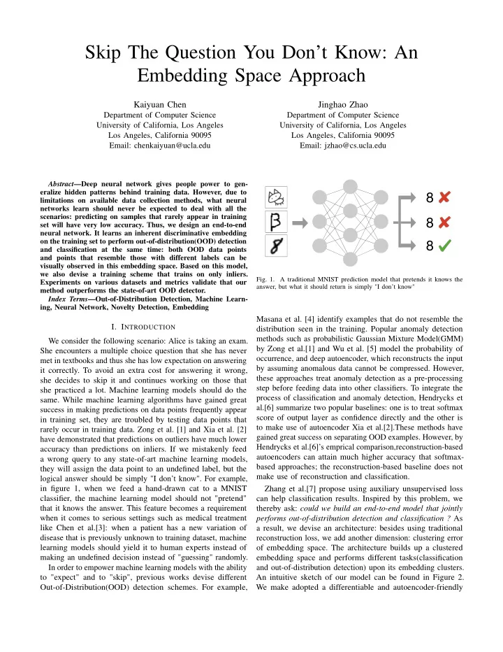
success in making predictions on data points frequently appear in training set, they are troubled by testing data points that rarely occur in training data. Zong et al. [1] and Xia et al. [2] have demonstrated that predictions on outliers have much lower accuracy than predictions on inliers. If we mistakenly feed a wrong query to any state-of-art machine learning models, they will assign the data point to an undefined label, but the logical answer should be simply "I don’t know". For example, in figure 1, when we feed a hand-drawn cat to a MNIST classifier, the machine learning model should not "pretend" that it knows the answer. This feature becomes a requirement when it comes to serious settings such as medical treatment like Chen et al.[3]: when a patient has a new variation of disease that is previously unknown to training dataset, machine learning models should yield it to human experts instead of making an undefined decision instead of "guessing" randomly. In order to empower machine learning models with the ability to "expect" and to "skip", previous works devise different Out-of-Distribution(OOD) detection schemes. For example,

8 8 8

• Fig. 1.

A traditional MNIST prediction model that pretends it knows the answer, but what it should return is simply "I don’t know"

Masana et al. [4] identify examples that do not resemble the distribution seen in the training. Popular anomaly detection methods such as probabilistic Gaussian Mixture Model(GMM) by Zong et al.[1] and Wu et al. [5] model the probability of

• ccurrence, and deep autoencoder, which reconstructs the input

by assuming anomalous data cannot be compressed. However, these approaches treat anomaly detection as a pre-processing step before feeding data into other classifiers. To integrate the process of classification and anomaly detection, Hendrycks et al.[6] summarize two popular baselines: one is to treat softmax score of output layer as confidence directly and the other is to make use of autoencoder Xia et al.[2].These methods have gained great success on separating OOD examples. However, by Hendrycks et al.[6]’s emprical comparison,reconstruction-based autoencoders can attain much higher accuracy that softmax- based approaches; the reconstruction-based baseline does not make use of reconstruction and classification. Zhang et al.[7] propose using auxiliary unsupervised loss can help classification results. Inspired by this problem, we thereby ask: could we build an end-to-end model that jointly performs out-of-distribution detection and classification ? As a result, we devise an architecture: besides using traditional reconstruction loss, we add another dimension: clustering error

• f embedding space. The architecture builds up a clustered

embedding space and performs different tasks(classification and out-of-distribution detection) upon its embedding clusters. An intuitive sketch of our model can be found in Figure 2. We make adopted a differentiable and autoencoder-friendly

clustering loss from Deep Embedding Clustering(DEC) by Xie et al.[8]. As demonstrated by Guo et al.[9], such an architecture preserves local structures of data points and clusters data points discriminatively, so our experiment shows its strong ability for classification and generative reconstruction to detect out-of- distribution outliers. In addition, we can visually backtrack data points that are classified as "novel" by our model, by which we can determine on whether this data point is an out-of-whole- distribution or it has stronger similarity to other clusters. This gives more interpretability than other autoencoder-based OOD detection methods. Our contributions of this work can be summarized as below:

• We propose an end-to-end architecture with associated loss

function that jointly optimizes out-of-distribution detection and classification by learning a label-clustered embedding

• We understand outliers by backtracking them visually in
• ur embedding space and devise a training process that

dynamically removes outliers in training set

• We empirically compare our model with other OOD

detection algorithms in various datasets that are mixed with OOD examples

• II. RELATED WORKS

In this section, we mainly introduce recent signs of progress on both softmax-based and reconstruction-based Out-

• f-Distribution Detection. We also present fundamental ideas

from Deep Embedding Clustering(DEC), which uses deep autoencoder to build up an embedding space in an unsupervised way.

• A. Out-of-Distribution Detection

Because deep neural network lacks interpretability and calibrated confidence estimates[9], Out-of-Distribution Detec- tion has drawn research attention in recent literature. Many approaches use the maximum value of the last activation function as a, typically softmax [6] to distinguish the outliers. A low maximum softmax probability usually indicates the data point is out of the distribution. For example, Liang et al.[10] use antiadversarial perturbation to the class with maximum probability and increase the softmax temperature. Devries et

• al. [11] slightly change the architecture by adding an auxiliary

branch to a classifier that outputs the OOD score from that

• branch. These approaches are simple to deploy because they

do not need to modify the original structure of the neural network; however, Hendrycks et al.[6] also show that using reconstruction based autoencoder can have close to 100 percent accuracy in datasets that softmax-approaches are tested on. Deep autoencoder is a feed-forward multi-layer neural network that maps high dimensional data points into a much lower dimensional space nonlinearly. Thus, we can write a deep autoencoder abstractly as a combination of two nonlinear functions fEN and fDE. The reconstructed output for a data point x is thus x′ = fDE(fEN(x)) and the training procedure is to minimize the difference between the reconstructed example and the example itself. Namely, min

fDE,fEN ||fDE(fEN(x)) − x||2 2

Because when data are mapped to low dimensional space, we assume anomalous data are not compressible and will result in large reconstruction error. Xia et al.[2] present strong empirical evidence on separating anomalous data points in an unsupervised way. Shah et al. [12] develop upon deep autoencoder and propose QSSAE, which combines a non- convex loss and a heavy-tailed distribution model to label the

• utliers,

Because OOD is usually taken as an auxiliary step instead of an end, using autoencoder alone cannot guarantee a successful result on classifier side, because low dimensional space does not preserve label information. Directly using embedding space for classification will result in lower accuracy. However, Zhang et al. [7] propose using an auxiliary decoder as unsupervised costs can sometimes increase the performance of classification. Based on this observation, Hendrycks et al. [6] propose an abnormality classifier that appends after the reconstruction decoder that classifies in-distribution and out-of-distribution samples based on the reconstructed value. Unfortunately, it does not rely on data points’ label information.

• B. Deep Embedding Clustering

Traditional clustering methods, for example k-means algo- rithm, are comprehensively summarized by Pimentel et al.[13]. A good embedding space gives good performance on further calculation on reconstruction and classification. Thus, Xie et

• al. [8] proposed a differentiable neural network optimization

scheme called Deep Embedding Clustering(DEC). DEC learns an embedding space by in an unsupervised way to optimize towrads target distribution that can improve cluster purity. After pre-training an autoencoder to reconstruct the original input, Xie et al. [8] discard the decoder and directly optimize the distance distribution P between embedding space and cluster centers with a target distribution Q by Kullback–Leibler(KL) divergence L = KL(P||Q) =

• i
• j

pij log pij qij Given the embedding space Z = {zi}n1+n2

i=1

, they first initialize a k-means clustering with centroids {µj}k

j=1, where k

is the number of clusters. Then they calculate a soft assignment

• f these embedded points to these clusters. They use Student’s

t-distribution’s metric P = {pij} to measure the distance between zi and centroid µj, i.e. qij = (1 + ||zi − µj||2/α)− α+1

2

• j′(1 + ||zi − µ′

j||2/α)− α+1

2

As suggested by Maaten et al.[14], we can set the degrees

• f freedom parameter alpha = 1 since learning is superfluous.

We set target distribution P given computed qij to be pij = q2

ij/ i qij

′

j q2 ij′/ i qij

Encoder Decoder Classifier

Reconstruction Error > ε? No Yes Images Embedding Space Reconstruction Images

Output: “I don’t know”

Output: 2

• Fig. 2. Our basic architecture that learns an embedding space that can perform both anomaly detection and classification at the same time

Intuitively, equation II-B normalize the frequency of each soft clusters to prevent embedding space distortion and Xie et al.[8] justify the target distribution formulation by using its partial derivatives to each embedded point: points closer to the center

• f the clusters will contribute more weights to gradients.
• III. METHODOLOGY

In this section, we describe the architecture and optimization procedure of our proposed approach.

• A. Problem Formulation

Consider a dataset distribution X1 with n1 examples and their associated labels {(x1

1, y1 1)...(x1 n, y1 n1)} and an anomaly

distribution X2 with n2 << n1 examples {(x2

1, ∗)...(x2 n2, ∗)}.

We mark labels of anomaly distribution as ∗ since we don’t want our model to assign any label to these data. Then for all ǫ, δ ∈ [0, 1], a successful OOD algorithm A with its classifier C trained with X1 ∪ X2 should have at least 1 − δ probability to identify x such that ❊(ℓ(C(x), y)) > ǫ where ❊(·) is the expectation function and ℓ is the loss function. We define ℓ = 1 if y = ∗.

• B. Architecture

Directly following from problem formulation, we aim to reduce both the number of times that we attempt to classify adversarial data points from X2 and reduce the number

• f times that classifiers make mistakes. Because we use

deep autoencoder to reconstruct the original input to detect anomaly points, we need a reconstruction loss Jr. As we discussed in section 2, directly optimizing reconstruction loss and classification loss potentially lack conciliation between reducing dimension and separating different labels. Thus, we design an extra clustering penalty term for embedding space. Along with the classification loss Jc, we have our loss function J = Jr + λ1Je + λ2Jc , where λ1 and λ2 are constants. We define each of the above loss functions in the following ways:

• Embedding loss: Since we already know the labels for

all the data points, we define the centers of each label cluster to be µ′

j =

1 |yi = j|

• k

✶(yi = j)zk After initializing the embedding space by k-means, we use an interpolation between previous soft label assignment and current true label center as our distance distribution, that is, qij = (1 + ||zi − (1 − α)µj − αµ′

j||2)−1

• j(1 + ||zi − (1 − α)µj − αµ′

j||2)−1

where α is a regularizer constant that controls between grouping data points with similar labels and grouping data points with similar features. We still use equation II-B for target distribution. As a result, we define our reconstruction loss to be the KL divergence between current distribution target distribution Je =

• i
• j

pijlog pij qij

• Reconstruction loss: Using the fact anomalous data cannot

be compressed by denoising autoencoder by Devries et al. [11], we compute the ell2 distance between the original input x and the reconstructed input fDE(fEN(x)) where fDE is the decoding function and fEN is the encoding function, i.e. Jr = ||x − fDE(fEN(x))||2

2

Although Xie et al.[8]’s DEC discard their decoder after pre-trainning an autoencoder, Guo et al.[9] improve DEC by proposing Improved Deep Embedding Cluster- ing(IDEC) by considering the reconstruction loss, because this loss can help preserving local structures of data generating distribution instead of distorting the embedded space.

• Classification loss: We use classification loss to penalize
• n classification error.

Although the main purpose of this penalty term is to map from data point to labels, by Hershey et al. [15], the classification loss can also be used to enlarge the distance

Input Image Reconstructed Image Classification

Embedding Space Encoder Decoder Classifier

• Fig. 3. Architecture

between clusters and shrink distance within clusters. In this case, we use categorical cross entropy which calculates the cross entropy of true labels after a softmax function.

• C. Optimization on embedding loss

We optimize equation III-B by stochastic gradient de- scent(SGD) with learning rate 0.01. We also set our lambda1 and λ2 to be balanced throughout the optimization. When we train on a batch with size n, we use a similar derivation as Xie et al. [8] of cluster weights and centers by ∂Je ∂zi =2

n

• j=1

K(1 + ||zi − (1 − α)µj − αµ′

j||2)−1

(1) (pij − qij)(zi − ((1 − α)µj − αµ′

j))

(2) and ∂Je ∂µj =2

n

• j=1

K(1 + ||zi − (1 − α)µj − αµ′

j||2)−1

(3) (pij − qij)(zi − ((1 − α)µj − αµ′

j))

(4) and softly assigned cluster center can directly follow from gradient descent, µj = µj − η n

n

• i=1

∂Jc ∂µj where η is the learning rate.

• D. Training

One important observation is that when we pretrain an autoencoder to get an initial embedding, we can use the same autoencoder to perform a primitive OOD detection. Unsu- pervisedly using autoencoder to separate out-of-distribution data points from original data points during training time has demonstrated good results by Xia et al.[2]. Concretely, we pretrain our autoencoder with part of clean MNIST dataset. As a result of this observation, after pretraining reconstruc- tion part of the neural network with some clean data, we can simply sift away those which have large reconstruction loss when we jointly train the classifier and reconstruction neural network: i.e. given a assumed threshold ǫ, we can filter out top ǫ% points and train on the rest. Since we continue updating

• ur cluster center and target distribution, data points that are

close to the threshold will dynamically move from one side to the other: thus even if some in-distribution points are assumed as OOD in the previous iteration, the model can still converge to incorporate these points. To summarize, we have the following algorithm 1. Algorithm 1 OOD during training Input: training dataset X with label vector y; update interval T; Abnormal proportion ǫ

1: initialize clusters by equation (III-B) 2: initialize training set X′ = X, label y′ = y 3: Pretrain an autoencoder with loss function (III-B) based

• n part of clean dataset

4: for each update interval do 5:

Reconstruction, classification, embedding ← model prediction

6:

Compute reconstruction error by equation (III-B) and let index set ✶ = {top ǫ% largest reconstruction error } if the dataset contains some outliers

7:

X′ = X − X✶

8:

y′ = y − y✶

9:

z′ = z − z✶

10:

Compute target distribution P by equation (III-B) and (II-B) from z′

11:

for i ∈ 1...T do

12:

Update Decoder fDE, EncoderfEN and Classifier C by X′ and y′ and target distribution P Through this training scheme, even the whole dataset is not clean enough, what we need is a small part of clean data in the dataset, and then the classifier will not be affected during the training process, which can make the classifier have higher accuracy.

• IV. EXPERIMENT
• A. Datasets

To evaluate the effectiveness of classification and out-of- distribution classification, we replicate the same experiment setting as which introduced by Hendrycks et al. [6] and Devries et al. [11]. They separate their dataset to be in-distribution dataset and out-of-distribution dataset. 1) In-Distribution Dataset: a) MNIST: MNIST dataset[16] is a dataset of handwritten digits, which has 60000 training images and 10000 testing

• images. For each of the image, it is a grey-scale 28×28 matrix

that belongs to 10 classes from 1 to 10. b) CIFAR-10: CIFAR-10[17] is a dataset that contains colored images with size 32 × 32. Each image belongs to one

• f ten classes like dog, cat, car. The training set is 50000

images and the testing set has 10000 images.

2) Out-of-Distribution Dataset: For the purpose of compar- ing with other state-of-art OOD detection datasets, we use the same setting as the baseline method proposed by Hendrycks et al. [6]. a) iSUN: iSUN dataset[18] contains 8925 scene images

• f 10 scene categories. All the images are from SUN dataset

and processed by downsampling to size 32 × 32, which we use as the OOD dataset for CIFAR-10. b) Omniglot: Omniglot dataset[19] contains handwritten characters rather than digits in MNIST. We use 10000 28 × 28 greyscale characters as the OOD dataset for MNIST. c) notMNIST: This dataset[20] contains 10000 28 × 28 images of letters from A to J on various typefaces. We use it as the OOD dataset for MNIST. d) CIFAR10-bw: This dataset is rescaled from CIFAR-10. It contains greyscale images of size 28×28 as the OOD dataset

• f MNIST.

e) noise: This dataset contains 10000 32 × 32 RGB or 28 × 28 greyscale(depends on the dataset used) images. Each pixel is sampled i.i.d from a uniform or Gaussian distribution and labels are assigned randomly from 1 to 10. f) MNIST-{x}: This dataset is generated from original MNIST dataset by removing points with label x. For ex- ample, MNIST-{0,1} means we use data points with label 2,3,4,5,6,7,8,9 as in-samples and points with label 0 and 1 as

• utliers.
• B. Evaluation Metrics

We measure the quality of out-of-distribution detection by metrics defined by Hendrycks et al. [6]. For choosing the novelty detection threshold according to the novelty score implies trade-off between the false negative and false positive, the following metrics can show the performance from different angles. a) AUROC: Area Under Receiver Operating Characteris- tic(AUROC) curve measure the area under Receiver Operating Characteristic(ROC) curve. It equals to the probility that the OOD detection classifier will rank a randomly chosen positive samples higher than a negative one. 100% AUROC score means that the OOD detection can perfectly distinguish the positive and negative examples. b) AUPR-In: Area Under Precision-Recall(AUPR) curve measures the area under Precision-Recall curve of out-of- distribution detection. The Precision-Recall curve plots the precision (TP/(TP+FP)) as the function of recall (TP/(TP+FN)). 100% AUPR score means that the classifier can perfectly distinguish the positive and negative examples. AUPR-In metric is the AUPR score when we treat the in-distribution images as positive samples. c) AUPR-Out: Just like the AUPR-In metric, AUPR-Out metric is the AUPR score when we treat the out-of-distribution images as positive samples.

• C. Experiment Results

In this section, We compare the performance of our model’s novelty detection with state-of-art novelty detection methods.

In-Distribution/ Out-of-Distribution AUROC AUPR-In AUPR-Out Hendrycks et al.[6]/Our Method CIFAR-10/SUN 99.99/100 99.95/100 99.04/100 CIFAR-10/Gaussian 100/100 100/100 99.24/100 MNIST/Omniglot 99.45/99.50 99.49/99.45 99.40/99.38 MNIST/notMNIST 100/100 100/100 99.97/100 MNIST/CIFAR-10bw 99.97/100 99.97/100 99.97/100 MNIST/Gaussian 100/100 100/100 100/100 MNIST/Uniform 100/100 100/100 100/100 TABLE I THE EVALUATION OF IN- AND OUT-OF-DISTRIBUTION DETECTION FOR THE

DATASETS IN BASELINE. THE BOLD TEXT INDICATES BETTER NOVELTY DETECTION PERFORMANCE. EACH VALUE CELL IS IN "BASELINE/OUR

METHOD" FORMAT. In-Distribution/ Out-of-Distribution AUROC AUPR-In AUPR-Out Hendrycks et al.[6]/Our Method MNIST’/MNIST-{0,1} 93.57/94.65 98.10/98.16 75.98/89.10 MNIST’/MNIST-{2,3} 90.46/98.85 96.44/99.72 75.48/95.18 MNIST’/MNIST-{4,5} 92.82/96.78 98.25/99.24 72.98/86.88 MNIST’/MNIST-{6,7} 95.37/95.49 98.76/98.81 82.90/84.13 MNIST’/MNIST-{8,9} 94.63/95.52 98.69/98.86 75.19/82.68 TABLE II THE EVALUATION OF IN- AND OUT-OF-DISTRIBUTION DETECTION FOR THE MNIST-X. THE BOLD TEXT INDICATES BETTER NOVELTY DETECTION

• PERFORMANCE. EACH VALUE CELL IS IN "BASELINE/OUR METHOD"

FORMAT.

Our results show that our method has higher novelty detection rates and better interpretability at the same time. To the best of authors’ knowledge, current state-of-art softmax-based approaches have not surpassed the benchmark for reconstruction based approaches. We shall directly compare with the reconstruction-based OOD detection deep autoencoder module proposed by Hendrycks et al. [6]. By using the datasets mentioned in section 4.A, our model passed the baseline tests

• n all benchmarks for CIFAR-10 and MNIST dataset that are

mixed with samples from other datasets, as showed in Table IV-C. However, baseline algorithm shows poor results when we use it in MNIST-x datasets. This result makes sense since its anomaly detection module only looks at the reconstruction and classification entropy, while it fails to consider the importance

• f discriminative labels in the encoded embedding space. The

comparison is shown in Table I. This observation is important since the difference between MNIST dataset and other out-sample datasets is large in terms

• f the position of digits, greyscale level and intrinsic structures.

However, in practical usage, the "out" samples are usually drawn from the dataset that comes from the same distribution as the training set, As a result, we claim that the examples from

• ther datasets are not as challenging as identifying that a new

label exists. In this experiment, our model still demonstrates descent results.

(a) Autoencoder (b) Autoencoder+Classifier (c) Autoencoder+Classifier+Cluster Loss

• Fig. 4. The comparison of embedding spaces of model that only uses autoencoder, model that uses autoencoder and classifier and our model. Our model

shows better cluster and classification performance.

• D. Embedding Visualization

One of our main features of our constructed embedding space is we can backtrace a single data point to know visually where it is in the embedding space. This allows us to analyze and diagnosis: 1) whether this point is out-of-distribution of the whole dataset. For example, how an OOD example behaves and why our model classifies it as OOD. 2) whether the data point is misclassied because this point is out-of-distribution of the label cluster it belongs to. For example, one might write an one that looks like a two, which are illustrated in Figure 5. This help us to understand why some samples are classified as OOD examples. The cluster penalization term in our method will make the distributions of normal samples at the embedding layer more representative. When an outlier comes, the difference of distributions at embedding layer will give higher reconstruction error, which helps us to distinguish the OOD samples. In

• rder to illustrate the importance of clustering loss, we make

a comparison of embedding spaces of model that only uses autoencoder, model that uses both autoencoder and classifier and our model in Figure 4. We use the dataset MNIST-{0,1} as an illustration: we first train all models with same set

• f hyperparameters, and evaluate the performance of OOD

by treating all 0 and 1 examples as outliers. To better show the generalizing power, we use testing dataset to draw their embedding spaces. As we can observe, the autoencoder’s embedding space has already had a structure of different clusters. Since the objective function for autoencoder is simply to reduce dimensionality, autoencoder simply groups similar points together without taking into account labels. Consequently, this embedding space has poor discriminative power. Then we compare the embedding space of our model with the one that conjuncts an autoencoder and a classifier. The model without clustering loss has poor ability to separate between cluster 4 and cluster 9, the inter-cluster distance between 3 and 5 is also very small. In contrast, our model has much cleaner embedding space. For the OOD samples with label 0 and 1, we can observe that they are well separated from other clusters, and the distance between different label clusters are much larger than the previous two Input Output

• Fig. 5. Three types of samples and their positions at enbedding space. (a)
• ut-of distribution samples (b) correctly classified in-distribution samples (c)

misclassified in-distribution samples.

• models. As a result, our model will give outliers a much higher

reconstruction loss.

• V. DISCUSSION

In this work, we takes a different and novel approach to perform OOD detection from other previous works. Instead of focusing heavily on interpreting the values of softmax activation functions, we maintain a well organized embedding space, and perform all the rest functions like classification and OOD detection based on this embedding space. As we have shown in the visualization of embedding space in previous section, detecting out-of-distribution examples and correctly classifying data points based on this clean embedding space should not be challenging for a machine learning model, while performing the same task on other spaces, like only using autoencoder

• r using both autoencoder and classifier requires much more

expressive power and has potential problem of overfitting. Because of a cleaner embedding space, we can perform much more tasks than other state-of-art algorithms in classification, reconstruction of original example from low dimensional space, visualizing and diagnosing misclassified and OOD examples. We make a comparison with other state-of-arts in Table V.

OOD Detection Joint Optimization for Classifi- cation Clustering Interpretable Embedding space ODIN [10]

• DEC [8]
• Shaol

et al.[21]

• O

Devries et al.[11]

• Hendrycks

et al.[6]

• Our model
• TABLE III

THE COMPARISON WITH OTHER STATE-OF-ARTS MODELS. THE LABEL

CHECK MEANS THE MODEL HAS THE CORRESPONDING PROPERTY, AND THE LABEL "O" MEANS THE MODEL PARTIALLY HAS THE CORRESPONDING PROPERTY.

There is one important future direction is this embedding method of OOD classification. In this paper, we simply select anomaly threshold based on reconstruction loss Jr, i.e. a point is OOD example if Jr > ǫ. However, this embedding space can offer us much more insights. Because it is already a well- clustered embedding space, for a data point, we can use another metric J(x) = Jr(x) + λℓ(x, µi) where ℓ is a distance metric and λ is a hyperparameter and µi is the cluster center that the point belongs to. Because the latter distance term is commonly used for anomaly detection algorithms, for example, k-means algorithm, which measures the point’s novelty by distance to cluster centers, this embedding space can naturally inherit such property and this metric has great potential to be incoperated in current scheme. However, in order to streamline our proposed approach, we leave this evaluation criterion as a future work.

• VI. CONCLUSION

In this paper, we propose an end-to-end neural network, which learns an inherent discriminative embedding to jointly perform out-of-distribution detection and classification at the same time. Through experiments, our models can outperform the state-of-art OOD detector on all the metrics. We also find

• riginal goals of OOD detection for most of the state-of-arts

are not as challenging as removing points with certain labels as

• ut samples. Furthermore, our model has better interpretability

than other methods by visualizing embedding space. Based

• n our model, we also devise a training scheme that trains on
• nly inliers, which can help the classifier to train the model

more accurately on the datasets that are not fine-labelled or contaminated by noises.

• VII. ACKNOWLEDGEMENT

We would like to thank Quanquan Gu for constructive discussions. REFERENCES

[1] B. Zong, Q. Song, M. R. Min, W. Cheng, C. Lumezanu, D. Cho, and

• H. Chen, “Deep autoencoding gaussian mixture model for unsupervised

anomaly detection,” 2018. [2] Y. Xia, X. Cao, F. Wen, G. Hua, and J. Sun, “Learning discriminative reconstructions for unsupervised outlier removal,” in Proceedings of the IEEE International Conference on Computer Vision, 2015, pp. 1511– 1519. [3] K. Chen, J. Shen, and F. Scalzo, “Skull stripping using confidence segmentation convolution neural network,” in International Symposium

• n Visual Computing.

Springer, 2018, pp. 15–24. [4] M. Masana, I. Ruiz, J. Serrat, J. van de Weijer, and A. M. Lopez, “Metric learning for novelty and anomaly detection,” arXiv preprint arXiv:1808.05492, 2018. [5] W. Wu, Y. Zheng, K. Chen, X. Wang, and N. Cao, “A visual analytics approach for equipment condition monitoring in smart factories of process industry,” in Pacific Visualization Symposium (PacificVis), 2018 IEEE. IEEE, 2018, pp. 140–149. [6] D. Hendrycks and K. Gimpel, “A baseline for detecting misclassified and out-of-distribution examples in neural networks,” arXiv preprint arXiv:1610.02136, 2016. [7] Y. Zhang, K. Lee, and H. Lee, “Augmenting supervised neural networks with unsupervised objectives for large-scale image classification,” in International Conference on Machine Learning, 2016, pp. 612–621. [8] J. Xie, R. Girshick, and A. Farhadi, “Unsupervised deep embedding for clustering analysis,” in International conference on machine learning, 2016, pp. 478–487. [9] X. Guo, L. Gao, X. Liu, and J. Yin, “Improved deep embedded clustering with local structure preservation,” in International Joint Conference on Artificial Intelligence (IJCAI-17), 2017, pp. 1753–1759. [10] S. Liang, Y. Li, and R. Srikant, “Enhancing the reliability of out-

• f-distribution image detection in neural networks,” arXiv preprint

arXiv:1706.02690, 2017. [11] T. DeVries and G. W. Taylor, “Learning confidence for out-of-distribution detection in neural networks,” arXiv preprint arXiv:1802.04865, 2018. [12] M. P. Shah, S. Merchant, and S. P. Awate, “Abnormality detection using deep neural networks with robust quasi-norm autoencoding and semi- supervised learning,” in Biomedical Imaging (ISBI 2018), 2018 IEEE 15th International Symposium on. IEEE, 2018, pp. 568–572. [13] M. A. Pimentel, D. A. Clifton, L. Clifton, and L. Tarassenko, “A review

• f novelty detection,” Signal Processing, vol. 99, pp. 215–249, 2014.

[14] L. Maaten, “Learning a parametric embedding by preserving local structure,” in Artificial Intelligence and Statistics, 2009, pp. 384–391. [15] J. R. Hershey, Z. Chen, J. Le Roux, and S. Watanabe, “Deep clustering: Discriminative embeddings for segmentation and separation,” in Acoustics, Speech and Signal Processing (ICASSP), 2016 IEEE International Conference on. IEEE, 2016, pp. 31–35. [16] L. Deng, “The mnist database of handwritten digit images for machine learning research [best of the web],” IEEE Signal Processing Magazine,

• vol. 29, no. 6, pp. 141–142, 2012.

[17] A. Krizhevsky, “Learning multiple layers of features from tiny images,” 2009. [18] J. Xiao, J. Hays, K. A. Ehinger, A. Oliva, and A. Torralba, “Sun database: Large-scale scene recognition from abbey to zoo,” in Computer vision and pattern recognition (CVPR), 2010 IEEE conference on. IEEE, 2010,

• pp. 3485–3492.

[19] B. M. Lake, R. Salakhutdinov, and J. B. Tenenbaum, “Human-level concept learning through probabilistic program induction,” Science, vol. 350, no. 6266, pp. 1332–1338, 2015. [20] Y. Bulatov, “Notmnist dataset,” Google (Books/OCR), Tech. Rep.[Online]. Available: http://yaroslavvb. blogspot. it/2011/09/notmnist-dataset. html, 2011. [21] X. Shaol, K. Ge, H. Su, L. Luo, B. Peng, and D. Li, “Deep Discriminative Clustering Network,” 2018 International Joint Conference

• n Neural Networks (IJCNN), pp. 1–7, 2018. [Online]. Available:

https://ieeexplore.ieee.org/document/8489417/