Fragile Separation Robust Separation x 2 x 2 x 2 x 2 New data x 1 - - PowerPoint PPT Presentation

1

Class #10: Kernel Functions and Support Vector Machines (SVMs)

Machine Learning (COMP 135): M. Allen, 07 Oct. 19

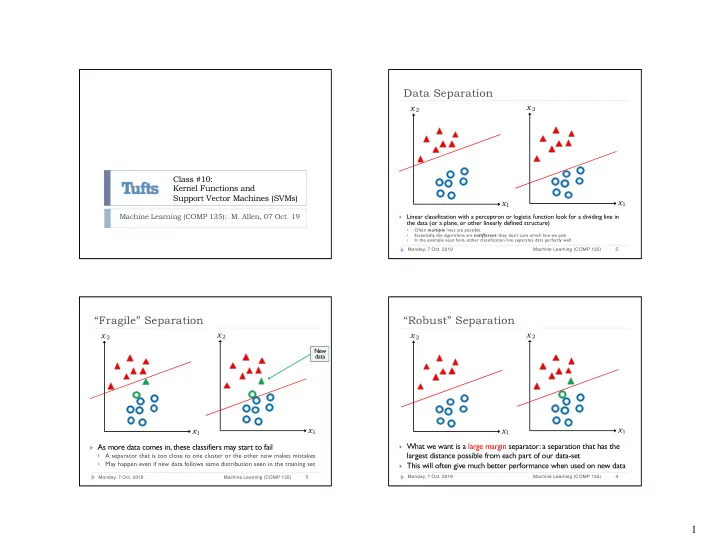
Data Separation

}

Linear classification with a perceptron or logistic function look for a dividing line in the data (or a plane, or other linearly defined structure)

}

Often multiple lines are possible

}

Essentially, the algorithms are indifferent: they don’t care which line we pick

}

In the example seen here, either classification line separates data perfectly well Monday, 7 Oct. 2019 Machine Learning (COMP 135) 2

x1 x 2 x1 x 2

“Fragile” Separation

} As more data comes in, these classifiers may start to fail } A separator that is too close to one cluster or the other now makes mistakes } May happen even if new data follows same distribution seen in the training set

Monday, 7 Oct. 2019 Machine Learning (COMP 135) 3

x1 x 2 x1 x 2

New data

“Robust” Separation

} What we want is a large margin separator: a separation that has the

largest distance possible from each part of our data-set

} This will often give much better performance when used on new data

Monday, 7 Oct. 2019 Machine Learning (COMP 135) 4

x1 x 2 x1 x 2

2 Large Margin Separation

} A new learning problem: find the separator with the largest margin } This will be measured from the data points, on opposite sides, that

are closest together

Monday, 7 Oct. 2019 Machine Learning (COMP 135) 5

x1 x 2

This is sometimes called the “widest road” approach A support vector machine (SVM) is a technique that finds this road. The points that define the edges

• f the road are the support

vectors. SVM Weight equation Threshold function

Linear Classifiers and SVMs

Monday, 7 Oct. 2019 Machine Learning (COMP 135) 6

Linear Weight equation Threshold function w · x = w0 + w1x1 + w2x2 + · · · + wnxn hw = ( 1 w · x ≥ 0 w · x < 0 hw = ( +1 w · x ≥ 0 −1 w · x < 0 w · x + b = (w1x1 + w2x2 + · · · + wnxn) + b

Large Margin Separation

} Like a linear classifier, the SVM separates at the line where its learned

vector of weights is zero

Monday, 7 Oct. 2019 Machine Learning (COMP 135) 7

x1 x 2

w · x + b = 0

+1 –1 A key difference: the SVM is going to do this without learning and remembering weight vector w. Instead, it will use features of the data-items themselves.

Mathematics of SVMs

} It turns out that the weight-vector w for the largest margin separator

has some important properties relative to the closest data-points on each side (x+ and x –)

Monday, 7 Oct. 2019 Machine Learning (COMP 135) 8

x1 x 2

x + x –

w · x+ + b = +1 w · x− + b = −1 w · (x+ − x−) = 2 w ||w|| · (x+ − x−) = 2 ||w|| ||w|| = q w2

1 + w2 2 + · · · + w2 n

3 Mathematics of SVMs

} Through the magic of mathematics (Lagrangian multipliers, to

be specific), we can derive a quadratic programming problem

1.

We start with our data-set:

2.

We then solve the constrained optimization problem:

Monday, 7 Oct. 2019 Machine Learning (COMP 135) 9

{(x1, y1), (x2, y2), . . . , (xn, yn)} [ ∀i, yi ∈ {+1, −1} ] W(α) = X

i

αi − 1 2 X

i,j

αi αj yi yj(xi · xj) ∀i, αi ≥ 0 X

i

αi yi = 0

The goal: based on known values ( ) find the values we don’t know (𝛽i ) that: 1. Will maximize value W(𝛽i) 2. Satisfy the two numerical constraints

xi, yi

Mathematics of SVMs

} The details of how all this is done are a bit complicated, but a

constrained optimization problem like this can be algorithmically solved to get all of the 𝛽i values needed:

} Once done, we can find the weight-vector and bias term if we want:

Monday, 7 Oct. 2019 Machine Learning (COMP 135) 10

W(α) = X

i

αi − 1 2 X

i,j

αi αj yi yj(xi · xj) ∀i, αi ≥ 0 X

i

αi yi = 0 w = X

i

αi yi xi b = −1 2( max

i | yi=−1 w · xi +

min

j | yj=+1 w · xj)

The Dual Formulation

} It turns out that we don’t need to use the weights at all } Instead, we can simply use the 𝛽i values directly: } Now, if we had to sum over every data-point like we do

• n the right-hand side of this equation, this would look

very bad for a large data-set

} It turns out that these 𝛽i values have a special property,

however, that makes it feasible to use them as part of our classification function…

Monday, 7 Oct. 2019 Machine Learning (COMP 135) 11

w · xi + b = X

j

αj yj (xi · xj) − b

Sparseness of SVMs

} The 𝛽i values are 0 everywhere except at the support vectors

(the points closest to the separator)

Monday, 7 Oct. 2019 Machine Learning (COMP 135) 12

x1 x 2

𝛽+ 𝛽 –

𝛽i = 0

This means that when we do the classification calculation: We only have to sum over points xj that are in the set of support vectors, ignoring all others. Thus, an SVM need only remember and use the values for the few support vectors, not those for all the rest of the data. X

j

αj yj (xi · xj) − b

4 Another Nice Trick

} The calculation uses dot-products of data-points with each

• ther (instead of with weights)

} This will allow us to deal with data that is not linearly separable

Monday, 7 Oct. 2019 Machine Learning (COMP 135) 13

x1 x 2

X

j

αj yj (xi · xj) − b Using a kernel “trick”, we can find a function that transforms the data into another form, where it is actually possible to separate it in a linear manner.

Transforming Non-Separable Data

} If data that is not linearly separable, we can transform it } We change features used to represent our data } Really, we don’t care what the data feature are, so long as we can get

classification to work

Monday, 7 Oct. 2019 Machine Learning (COMP 135) 14

x1 x 2

A transformation function: maps data-vectors to new vectors, of either the same dimensionality (m = n) or a different one (m ≠ n)

ϕ(x) ϕ : Rn → Rm

Transforming Non-Separable Data

Monday, 7 Oct. 2019 Machine Learning (COMP 135) 15

x 2 x1

ϕ(x) ϕ : Rn → Rm

x 2 x1

ϕ( ) ϕ( ) ϕ( ) ϕ( ) ϕ( ) ϕ( ) ϕ( ) ϕ( ) ϕ( ) ϕ( )

X

j

αj yj (ϕ(xi) · ϕ(xj)) − b

The “Kernel Trick”

Monday, 7 Oct. 2019 Machine Learning (COMP 135) 16

• 1.5
• 1
• 0.5

0.5 1 1.5

• 1.5
• 1
• 0.5

0.5 1 1.5 x2 x1 0.5 1 1.5 2 x1

2

0.5 1 1.5 2 2.5 x2

2

• 3
• 2
• 1

1 2 3 √2x1x2

(a) (b)

ϕ(x1, x2) = (x2

1, x2 2,

√ 2x1x2)

Image source: Russel & Norvig, AI: A Modern Approach (Prentice Hal, 2010)

5

} We can derive a simpler (2-dimensional) equation, equivalent

to the cross-product needed when doing SVM computations in the transformed (3-dimensional) space: ϕ(x) · ϕ(z) = (x2

1, x2 2,

√ 2x1x2) · (z2

1, z2 2,

√ 2z1z2) = x2

1z2 1 + x2 2z2 2 +

√ 2x1x2 √ 2z1z2 = x2

1z2 1 + x2 2z2 2 + 2x1x2z1z2

= (x1z1 + x2z2)2 = (x · z)2

Simplifying the Transformation Function

Monday, 7 Oct. 2019 Machine Learning (COMP 135) 17

10 multiplications 2 additions

3 multiplications 1 addition

Needed Used instead

The Kernel Function

} This final function (right side) is what the SVM will

actually use to compute dot-products in its equations

} This is called the kernel function } To make SVMs really useful we look for a kernel that: 1.

Separates the data usefully

2.

Is relatively efficient to calculate

Monday, 7 Oct. 2019 Machine Learning (COMP 135) 18

k(x, z) = ϕ(x) · ϕ(z) = (x · z)2

This Week

} T

• day: Kernels and SVMs

} Readings: Linked from class website schedule page. } Homework 03: due Wednesday, 16 October, 9:00 AM } Office Hours: 237 Halligan, Tuesday, 11:00 AM – 1:00 PM

} TA hours can be found on class website as well

Monday, 7 Oct. 2019 Machine Learning (COMP 135) 19