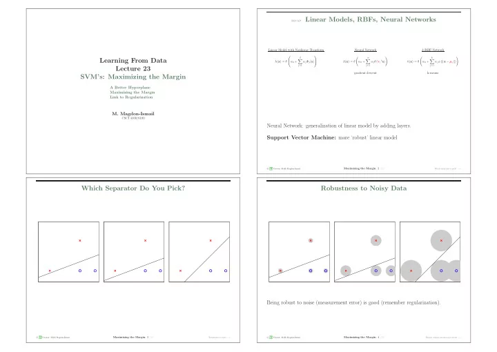
recap: Linear Models, RBFs, Neural Networks Linear Model with - PowerPoint PPT Presentation

recap: Linear Models, RBFs, Neural Networks Linear Model with Nonlinear Transform Neural Network k -RBF-Network   � � � � ˜ d m k Learning From Data � � � h ( x ) = θ  w 0 + w j Φ j ( x ) h ( x ) = θ w 0 + w j θ ( v j t x ) h ( x ) = θ w 0 + w j φ ( | | x − µ j | | )  j =1 j =1 j =1 Lecture 23 gradient descent k-means SVM’s: Maximizing the Margin A Better Hyperplane Maximizing the Margin Link to Regularization M. Magdon-Ismail CSCI 4100/6100 Neural Network: generalization of linear model by adding layers. Support Vector Machine: more ‘robust’ linear model � A M Maximizing the Margin : 2 /19 c L Creator: Malik Magdon-Ismail Which separator to pick? − → Which Separator Do You Pick? Robustness to Noisy Data Being robust to noise (measurement error) is good (remember regularization). Being robust to noise (measurement error) is good (remember regularization). � A c M Maximizing the Margin : 3 /19 � A c M Maximizing the Margin : 4 /19 L Creator: Malik Magdon-Ismail Robustness to noise − → L Creator: Malik Magdon-Ismail Thicker cushion means more robust − →

Thicker Cushion Means More Robustness Two Crucial Questions 1. Can we efficiently find the fattest separating hyperplane? 2. Is a fatter hyperplane better than a thin one? We call such hyperplanes fat � A M Maximizing the Margin : 5 /19 � A M Maximizing the Margin : 6 /19 c L Creator: Malik Magdon-Ismail Two crucial questions − → c L Creator: Malik Magdon-Ismail Pulling out the bias − → Pulling Out the Bias Separating The Data Hyperplane h = ( b, w ) Before Now h separates the data means: w t x n + b > 0 y n ( w t x n + b ) > 0 x ∈ { 1 } × R d ; w ∈ R d +1 x ∈ R d ; b ∈ R , w ∈ R d     bias b 1 w 0     By rescaling the weights and bias, x 1 w 1 x 1 w 1     x =  ; w =  .  .   .  . . . . .  ; .  . . . x = . w = .     n =1 ,...,N y n ( w t x n + b ) = 1 min x d w d x d w d w t x n + b < 0 signal = w t x signal = w t x + b (renormalize the weights so that the signal w t x + b is meaningful) � A c M Maximizing the Margin : 7 /19 � A c M Maximizing the Margin : 8 /19 L Creator: Malik Magdon-Ismail Separating the data − → L Creator: Malik Magdon-Ismail Distance to the hyperplane − →

Distance to the Hyperplane Fatness of a Separating Hyperplane 1 w is normal to the hyperplane: dist ( x , h ) = | · | w t x + b | | | w | w t ( x 2 − x 1 ) = w t x 2 − w t x 1 = − b + b = 0 . x (because w t x = − b on the hyperplane) w Unit normal u = w / | | w | | . dist ( x , h ) Since | w t x n + b | = | y n ( w t x n + b ) | = y n ( w t x n + b ) , Fatness = Distance to the closest point x 2 1 dist ( x n , h ) = | · y n ( w t x n + b ) . | | w | x 1 dist ( x , h ) = | u t ( x − x 1 ) | 1 Fatness = min n dist ( x n , h ) = | · | w t x − w t x 1 | | | w | 1 n y n ( w t x n + b ) = | · min ← − separation condition | | w | 1 | · | w t x + b | = 1 | | w | = ← − the margin γ ( h ) | | w | | � A M Maximizing the Margin : 9 /19 � A M Maximizing the Margin : 10 /19 c L Creator: Malik Magdon-Ismail Fatness of a separating hyperplane − → c L Creator: Malik Magdon-Ismail Maximizing the margin − → Maximizing the Margin Maximizing the Margin 1 margin γ ( h ) = ← − bias b does not appear here 1 margin γ ( h ) = ← − bias b does not appear here | | w | | | | w | | 1 minimize 2 w t w 1 minimize 2 w t w b, w b, w subject to: n =1 ,...,N y n ( w t x n + b ) = 1 . min subject to: n =1 ,...,N y n ( w t x n + b ) = 1 . min 1 minimize 2 w t w 1 minimize 2 w t w b, w b, w subject to: y n ( w t x n + b ) ≥ 1 for n = 1 , . . . , N. subject to: y n ( w t x n + b ) ≥ 1 for n = 1 , . . . , N. � A c M Maximizing the Margin : 11 /19 � A c M Maximizing the Margin : 12 /19 L Creator: Malik Magdon-Ismail Equivalent form − → L Creator: Malik Magdon-Ismail Example – our toy data set − →

Example – Our Toy Data Set Quadratic Programming y n ( w t x n + b ) ≥ 1     0 0 − 1 − b ≥ 1 ( i ) 2 2 − 1 − (2 w 1 + 2 w 2 + b ) ≥ 1 ( ii )     1 X = y = minimize 2 u t Q u + p t u     2 0 +1 2 w 1 + b ≥ 1 ( iii )     u ∈ R q 3 0 +1 3 w 1 + b ≥ 1 ( iv ) subject to: A u ≥ c (i) and (iii) gives w 1 ≥ 1 (ii) and (iii) gives w 2 ≤ − 1 So, 1 2 ( w 2 1 + w 2 2 ) ≥ 1 ( b = − 1 , w 1 = 1 , w 2 = − 1) u ∗ ← QP (Q , p , A , c ) Optimal Hyperplane 0 . 707 g ( x ) = sign( x 1 − x 2 − 1) 1 | = 1 √ margin: 2 ≈ 0 . 707 . 0 | w ∗ | | = 1 − x 2 − For data points (i), (ii) and (iii) y n ( w ∗ t x n + b ∗ ) = 1 x 1 ↑ Support Vectors (Q = 0 is linear programming) � A M Maximizing the Margin : 13 /19 � A M Maximizing the Margin : 14 /19 c L Creator: Malik Magdon-Ismail Quadratic programming − → c L Creator: Malik Magdon-Ismail Maximum margin hyperplane is QP − → Maximum Margin Hyperplane is QP Back To Our Example Exercise: 1 minimize 2 w t w y n ( w t x n + b ) ≥ 1 1 minimize 2 u t Q u + c t u b, w     u ∈ R q 0 0 − 1 − b ≥ 1 ( i ) subject to: A u ≥ a 2 2 − 1 − (2 w 1 + 2 w 2 + b ) ≥ 1 ( ii )     subject to: y n ( w t x n + b ) ≥ 1 for n = 1 , . . . , N. X = y =     2 0 +1 2 w 1 + b ≥ 1 ( iii )     3 0 +1 3 w 1 + b ≥ 1 ( iv ) Show that � � b     ∈ R d +1 u = − 1 0 0 1 w     0 0 0 0 − 1 − 2 − 2 1     Q = 0 1 0 p = 0 A = c =         1 2 0 1     0 0 1 0 1 3 0 1 w t � � � � � � � � � 1 0 b 0 0 � b 0 t 0 t 0 t d d d 2 w t w = = u t u = ⇒ Q = , p = 0 d +1 0 d I d w t 0 d I d 0 d I d Use your QP-solver to give         y 1 y 1 x t 1 y 1 y 1 x t 1 ( b ∗ , w ∗ 1 , w ∗ 1 1 2 ) = ( − 1 , 1 , − 1) . . . . . . � y n �  =  , c = . .  u ≥ . . . . y n ( w t x n + b ) ≥ 1 ≡ y n x t u ≥ 1 = ⇒ ⇒ A =  . .  .  . .  .  n y N y N x t 1 y N y N x t 1 N N � A c M Maximizing the Margin : 15 /19 � A c M Maximizing the Margin : 16 /19 L Creator: Malik Magdon-Ismail Back to our example − → L Creator: Malik Magdon-Ismail Primal QP algorithm − →

Primal QP algorithm for linear-SVM Example: SVM vs PLA 1: Let p = 0 d +1 be the ( d + 1)-vector of zeros and c = 1 N the N -vector of ones. Construct matrices Q and A, where E out (SVM)   � 0 y 1 — y 1 x t 1 — � 0 t . . . . d A = . . , Q =   0 d I d y N — y N x t N — � �� � signed data matrix � b ∗ � = u ∗ ← QP (Q , p , A , c ) . 2: Return w ∗ 0 . 04 0 0 . 02 0 . 06 0 . 08 E out 3: The final hypothesis is g ( x ) = sign( w ∗ t x + b ∗ ). PLA depends on the ordering of data (e.g. random) � A M Maximizing the Margin : 17 /19 � A M Maximizing the Margin : 18 /19 c L Creator: Malik Magdon-Ismail Example: SVM vs PLA − → c L Creator: Malik Magdon-Ismail Link to regularization Link to Regularization minimize E in ( w ) w subject to: w t w ≤ C. optimal hyperplane regularization minimize E in w t w subject to E in = 0 w t w ≤ C � A c M Maximizing the Margin : 19 /19 L Creator: Malik Magdon-Ismail