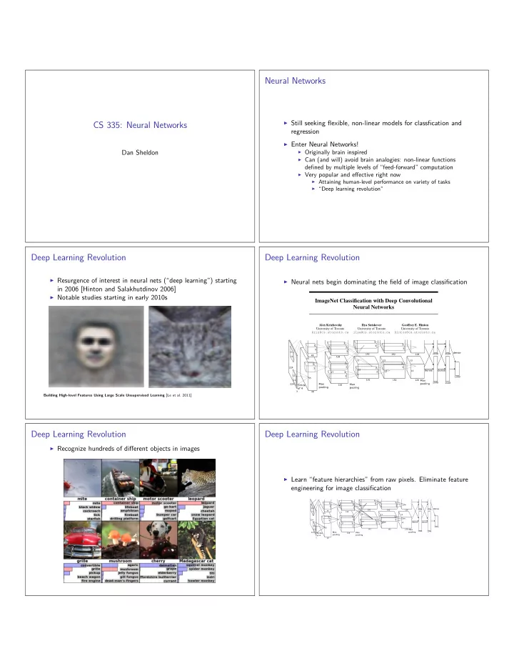
Neural Networks Still seeking flexible, non-linear models for - PDF document

Neural Networks ◮ Still seeking flexible, non-linear models for classfication and CS 335: Neural Networks regression ◮ Enter Neural Networks! ◮ Originally brain inspired Dan Sheldon ◮ Can (and will) avoid brain analogies: non-linear functions defined by multiple levels of “feed-forward” computation ◮ Very popular and effective right now ◮ Attaining human-level performance on variety of tasks ◮ “Deep learning revolution” Deep Learning Revolution Deep Learning Revolution ◮ Resurgence of interest in neural nets (“deep learning”) starting ◮ Neural nets begin dominating the field of image classification in 2006 [Hinton and Salakhutdinov 2006] ◮ Notable studies starting in early 2010s ImageNet Classification with Deep Convolutional Neural Networks Alex Krizhevsky Ilya Sutskever Geoffrey E. Hinton University of Toronto University of Toronto University of Toronto kriz@cs.utoronto.ca ilya@cs.utoronto.ca hinton@cs.utoronto.ca Building High-level Features Using Large Scale Unsupervised Learning [Le et al. 2011] Deep Learning Revolution Deep Learning Revolution ◮ Recognize hundreds of different objects in images ◮ Learn “feature hierarchies” from raw pixels. Eliminate feature engineering for image classification Lyle H Ungar, University of Pennsylvania

Deep Learning Revolution ◮ Deep learning has revolutionized the field of computer vision (image classfication, etc.) in last 7 years ◮ It is having a similar impact in other domains: ◮ Speech recognition ◮ Natural language processing ◮ Etc. Some History Why Now? ◮ “Shallow” networks in hardware: late 1950s ◮ Perceptron: Rosenblatt ~1957 ◮ Adaline/Madaline: Widrow and Hoff ~1960 ◮ Ideas have been around for many years. Why did “revolution” ◮ Backprop (key algorithmic principle) popularized in 1986 by happen so recently? Rumelhart et al. ◮ “Convolutional” neural networks: “LeNet” [LeCun et al. 1998] ◮ Massive training sets (e.g. 1 million images) ◮ Computation: GPUs ◮ Tricks to avoid overfitting, improve training Handwritten digit recognition C3: f. maps 16@10x10 C1: feature maps S4: f. maps 16@5x5 INPUT 6@28x28 32x32 S2: f. maps C5: layer F6: layer OUTPUT 6@14x14 120 10 84 3-nearest-neighbor = 2.4% error Gaussian connections 400–300–10 unit MLP = 1.6% error Full connection Convolutions Subsampling Convolutions Subsampling Full connection LeNet: 768–192–30–10 unit MLP = 0.9% error What is a Neural Network? Neural Networks: Key Conceptual Ideas ◮ Biological view: a model of neurons in the brain 1. Feed-forward computation ◮ Mathematical view 2. Backprop (compute gradients) ◮ Flexible class of non-linear functions with many parameters 3. Stochastic gradient descent ◮ Compositional: sequence of many layers ◮ Easy to compute Today: feed-forward computation and backprop ◮ h ( x ) : “feed-forward” ◮ ∇ θ h ( x ) : “backward propagation”

Feed-Forward Computation Feed-Forward Computation Multi-class logistic regression: Multiple layers h W, b ( x ) = W x + b W 1 ∈ R n 2 × n 1 , b 1 ∈ R n 2 h ( x ) = W 2 · g ( W 1 x + b 1 ) + b 2 , Parameters: W 2 ∈ R c × n 2 , b 2 ∈ R c ◮ W ∈ R c × n weights ◮ b ∈ R c biases / intercepts ◮ g ( · ) = nonlinear tranformation (e.g., logistic). “nonlinearity” ◮ h = g ( W 1 x + b 1 ) ∈ R d = “hidden” layer Output: draw picture ◮ h ( x ) ∈ R c = vector of class scores (before logistic transform) ◮ Q: why do we need g ( · ) ? draw picture Deep Learning Feed-Forward Computation General idea ◮ Write down complex models composed of many layers ◮ Linear tranformations (e.g., W 1 x + b ) � � f ( x ) = W 3 · g W 2 · g ( W 1 x + b 1 ) + b 2 + b 3 ◮ Non-linearity g ( · ) ◮ Write down loss function for outputs ◮ Optimize by (some flavor of) gradient descent How to compute gradient? Backprop! Backprop Backprop: Details Input variables v 1 , . . . , v k Assigned variables v k +1 , . . . , v n (includes ouput) Forward propagation : ◮ Boardwork: computation graphs, forward propagation, ◮ For j = k + 1 to n backprop ◮ v j = φ j ( · · · ) (local function of predecessors v i : i → j ) ◮ Code demos v i = dv n Backward propagation : compute ¯ dv i for all i ◮ Initialize ¯ v n = 1 ◮ Initialize ¯ v i = 0 for all i < n ◮ For j = n down to k + 1 ◮ For all i such that i → j ◮ ¯ d v i += dv i φ j ( · · · ) · ¯ v j

Stochastic Gradient Descent (SGD) Stochastic Gradient Descent (SGD) Algorithm Setup ◮ Initialize θ arbitrarily ◮ Complex model h θ ( x ) with parameters θ ◮ Repeat ◮ Cost function ◮ Pick random batch B ◮ Update m J ( θ ) = 1 cost ( h θ ( x ( i ) ) , y ( i ) ) � θ ← θ − α · 1 � ∇ θ cost ( h θ ( x ( i ) ) , y ( i ) ) m | B | i =1 i ∈ B 1 � cost ( h θ ( x ( i ) ) , y ( i ) ) ≈ ◮ In practice, randomize order of training examples and process | B | i ∈ B sequentially ◮ B = random “batch” of training examples (e.g., ◮ Discuss. Advantages of SGD? | B | ∈ { 50 , 100 , . . . } ), or even a single example ( | B | = 1 ) Stochastic Gradient Descent Discussion: Summary How do we use Backprop to train a Neural Net? ◮ Idea: think of neural network as a feed-forward model to compute cost ( h θ ( x ( i ) ) , y ( i ) ) for a single training example ◮ This is the same as gradient descent, except we approximate ◮ Append node for cost of prediction on x ( i ) to final outputs of the gradient using only training examples in batch network ◮ It lets us take many steps for each pass through the data set ◮ Illustration instead of one. ◮ Use backprop to compute ∇ θ cost ( h θ ( x ( i ) ) , y ( i ) ) ◮ In practice, much faster for large training sets (e.g., m = 1 , 000 , 000 ) ◮ This is all there is conceptually, but there are a many implementation details and tricks to do this effectively and efficiently. These are accessible to you, but outside the scope of this class. The Future of ML: Design Models, Not Algorithms ◮ Backprop can be automated! ◮ You specify the model and loss function ◮ Optimizer (e.g., SGD) computes gradient and updates model parameters ◮ Suggestions: autograd, PyTorch ◮ Demo: train a neural net with autograd ◮ Next steps ◮ Learn more about neural network architectures examples: other slides ◮ Code a fully connected neural network with one or two hidden layers yourself ◮ Experiment with more complex architectures using autograd or PyTorch