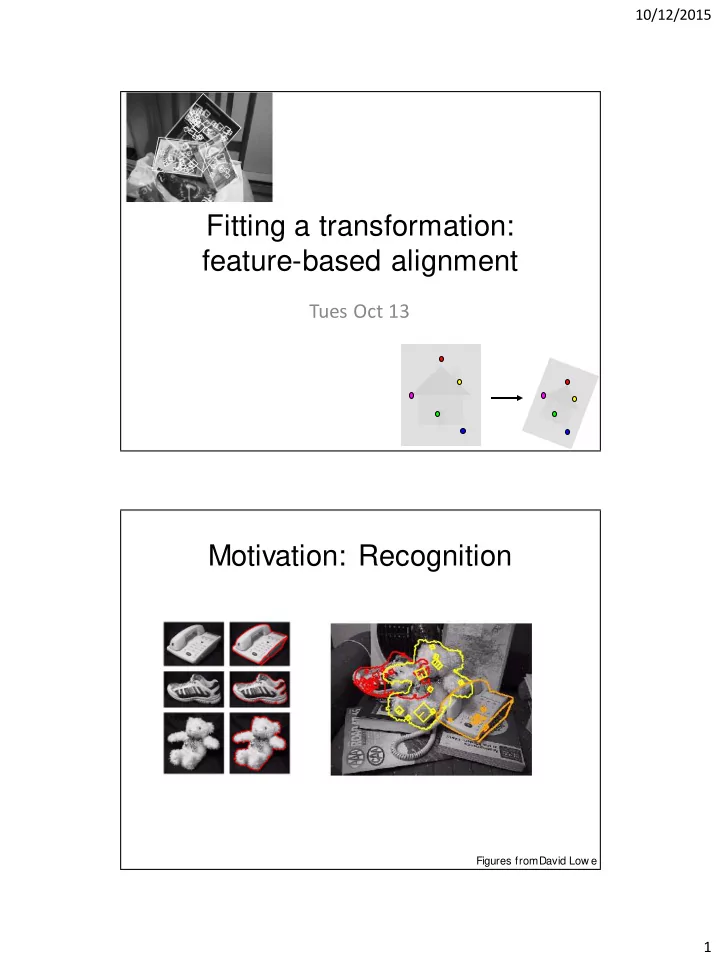
Fitting a transformation: feature-based alignment Tues Oct 13 - - PDF document

10/12/2015 1

Fitting a transformation: feature-based alignment

Tues Oct 13

Motivation: Recognition

Figures from David Low e

10/12/2015 2

Motivation: medical image registration Motivation: mosaics

Image f rom http://graphics.cs.cmu.edu/courses/15-463/2010_f all/

10/12/2015 3

Last week

• Interest point detection

– Harris corner detector – Laplacian of Gaussian, automatic scale selection

• Invariant descriptors

– Rotation according to dominant gradient direction – Histograms for robustness to small shifts and translations (SIFT descriptor)

Review questions

• What is the purpose of the “ratio test” for local

feature matching?

• What aspects of the SIFT descriptor design

promote robustness to lighting changes? Robustness to rotation and translation?

• Does extracting multiple keypoints for multiple

local maxima in scale space help recall or precision during feature matching?

• How far in the image plane can an object rotate

before the SIFT descriptors will not match?

10/12/2015 4

Multi-view: what’s next

Additional questions we need to address to achieve these applications:

• Fitting a parametric transformation given putative

matches

• Dealing with outlier correspondences
• Exploiting geometry to restrict locations of possible

matches

• Triangulation, reconstruction
• Efficiency when indexing so many keypoints

Coming up: robust feature-based alignment

Source: L. Lazebnik

10/12/2015 5

• Extract features

Source: L. Lazebnik

Coming up: robust feature-based alignment

• Extract features
• Compute putative matches

Source: L. Lazebnik

Coming up: robust feature-based alignment

10/12/2015 6

• Extract features
• Compute putative matches
• Loop:
• Hypothesize transformation T (small group of putative

matches that are related by T)

Source: L. Lazebnik

Coming up: robust feature-based alignment

• Extract features
• Compute putative matches
• Loop:
• Hypothesize transformation T (small group of putative

matches that are related by T)

• Verify transformation (search for other matches consistent

with T)

Source: L. Lazebnik

Coming up: robust feature-based alignment

10/12/2015 7

• Extract features
• Compute putative matches
• Loop:
• Hypothesize transformation T (small group of putative

matches that are related by T)

• Verify transformation (search for other matches consistent

with T)

Source: L. Lazebnik

Coming up: robust feature-based alignment

Today

• Feature-based alignment

– 2D transformations – Affine fit – RANSAC for robust fitting

10/12/2015 8

Alignment as fitting

• Previous lectures: fitting a model to features in one image
• Alignment: fitting a model to a transformation between

pairs of features (matches) in two images



i i M

x ) , ( residual





i i i

x x T ) ), ( ( residual

Find model M that minimizes Find transformation T that minimizes

M xi T xi xi

'

Slide credit: Lana Lazebnik

Parametric (global) warping

Examples of parametric warps:

translation rotation aspect affine perspective

Source: Alyosha Efros

10/12/2015 9

Parametric (global) warping

Transformation T is a coordinate-changing machine: p’ = T(p) What does it mean that T is global?

• Is the same for any point p
• can be described by just a few numbers (parameters)

Let’s represent T as a matrix: p’ = Mp T p = (x,y) p’ = (x’,y’)

             y x y x M ' '

Source: Alyosha Efros

Scaling

Scaling a coordinate means multiplying each of its components by a scalar Uniform scaling means this scalar is the same for all components:

 2

Source: Alyosha Efros

10/12/2015 10

Non-uniform scaling: different scalars per component:

Scaling

X  2, Y  0.5

Source: Alyosha Efros

Scaling

Scaling operation: Or, in matrix form:

by y ax x   ' '                    y x b a y x ' '

scaling matrix S

Source: Alyosha Efros

10/12/2015 11

What transformations can be represented with a 2x2 matrix?

2D Rotate around (0,0)?

y x y y x x * cos * sin ' * sin * cos '        

                        y x y x cos sin sin cos ' '

2D Shear?

y x sh y y sh x x

y x

    * ' * '

                   y x sh sh y x

y x

1 1 ' '

Source: Alyosha Efros

2D Scaling?

y s y x s x

y

x

* ' * '  

                   y x s s y x

y x

' '

What transformations can be represented with a 2x2 matrix?

Source: Alyosha Efros

2D Mirror about Y axis?

y y x x    ' '

                   y x y x 1 1 ' '

2D Mirror over (0,0)?

y y x x     ' '

                     y x y x 1 1 ' '

2D Translation?

y x

t y y t x x     ' '

NO!

10/12/2015 12

2D Linear Transformations

Only linear 2D transformations can be represented with a 2x2 matrix. Linear transformations are combinations of …

• Scale,
• Rotation,
• Shear, and
• Mirror

                   y x d c b a y x ' '

Source: Alyosha Efros

Homogeneous coordinates

homogeneous image coordinates

Converting from homogeneous coordinates To convert to homogeneous coordinates:

10/12/2015 13

Homogeneous Coordinates

Q: How can we represent 2d translation as a 3x3 matrix using homogeneous coordinates? A: Using the rightmost column:

           1 1 1

y x

t t ranslation T

y x

t y y t x x     ' '

Source: Alyosha Efros

Translation

                                            1 1 1 1 1 1 ' '

y x y x

t y t x y x t t y x

tx = 2 ty = 1 Homogeneous Coordinates

Source: Alyosha Efros

10/12/2015 14

Basic 2D Transformations

Basic 2D transformations as 3x3 matrices

                                    1 1 cos sin sin cos 1 ' ' y x y x                                1 1 1 1 1 ' ' y x t t y x

y x

                               1 1 1 1 1 ' ' y x sh sh y x

y x

Translate Rotate Shear

                               1 1 1 ' ' y x s s y x

y x

Scale

Source: Alyosha Efros

2D Affine Transformations

Affine transformations are combinations of …

• Linear transformations, and
• Translations

Parallel lines remain parallel                                w y x f e d c b a w y x 1 ' ' '

10/12/2015 15

Today

• Feature-based alignment

– 2D transformations – Affine fit – RANSAC for robust fitting

Alignment problem

• We have previously considered how to fit a model to

image evidence

– e.g., a line to edge points, or a snake to a deforming contour

• In alignment, we will fit the parameters of some

transformation according to a set of matching feature pairs (“correspondences”). T xi xi

'

10/12/2015 16

Image alignment

• Two broad approaches:

– Direct (pixel-based) alignment

• Search for alignment where most pixels agree

– Feature-based alignment

• Search for alignment where extracted features agree
• Can be verified using pixel-based alignment

Let’s start with affine transformations

• Simple fitting procedure (linear least squares)
• Approximates viewpoint changes for roughly planar
• bjects and roughly orthographic cameras
• Can be used to initialize fitting for more complex

models

Lana Lazebnik

10/12/2015 17

Fitting an affine transformation

• Assuming we know the correspondences, how do we

get the transformation?

) , (

i i y

x   ) , (

i i y

x

                           

2 1 4 3 2 1

t t y x m m m m y x

i i i i

An aside: Least Squares Example

Say we have a set of data points (X1,X1’), (X2,X2’), (X3,X3’), etc. (e.g. person’s height vs. weight) We want a nice compact formula (a line) to predict X’s from Xs: Xa + b = X’ We want to find a and b How many (X,X’) pairs do we need? What if the data is noisy?

' 2 2 ' 1 1

X b a X X b a X                       

' 2 ' 1 2 1

1 1 X X b a X X

Ax=B

                               ... ... ... 1 1 1

' 3 ' 2 ' 1 3 2 1

X X X b a X X X

• verconstrained

2

min B Ax 

Source: Alyosha Efros

10/12/2015 18

Fitting an affine transformation

• Assuming we know the correspondences, how do we

get the transformation?

) , (

i i y

x   ) , (

i i y

x

                           

2 1 4 3 2 1

t t y x m m m m y x

i i i i

                                                  

i i i i i i

y x t t m m m m y x y x

2 1 4 3 2 1

1 1

Fitting an affine transformation

• How many matches (correspondence pairs) do we

need to solve for the transformation parameters?

• Once we have solved for the parameters, how do we

compute the coordinates of the corresponding point for ?

• Where do the matches come from?

                                                  

i i i i i i

y x t t m m m m y x y x

2 1 4 3 2 1

1 1

) , (

new new y

x

10/12/2015 19

http://www.vlfeat.org/overview/sift.html Interest points and their scales and orientations (random subset of 50) SIFT descriptors

Recall: Scale Invariant Feature Transform (SIFT) descriptor [Lowe 2004]

Recall: SIFT (preliminary) matches

http://www.vlfeat.org/overview/sift.html

10/12/2015 20

Fitting an affine transformation

Figures from David Low e, ICCV 1999

Affine model approximates perspective projection of planar objects.

Today

• Feature-based alignment

– 2D transformations – Affine fit – RANSAC for robust fitting

10/12/2015 21

Outliers

• Outliers can hurt the quality of our parameter

estimates, e.g.,

– an erroneous pair of matching points from two images – an edge point that is noise, or doesn’t belong to the line we are fitting.

Outliers affect least squares fit

10/12/2015 22

Outliers affect least squares fit RANSAC

• RANdom Sample Consensus
• Approach: we want to avoid the impact of outliers,

so let’s look for “inliers”, and use those only.

• Intuition: if an outlier is chosen to compute the

current fit, then the resulting line (transformation) won’t have much support from rest of the points (matches).

10/12/2015 23

RANSAC for line fitting

Repeat N times:

• Draw s points uniformly at random
• Fit line to these s points
• Find inliers to this line among the remaining

points (i.e., points whose distance from the line is less than t)

• If there are d or more inliers, accept the line

and refit using all inliers

Lana Lazebnik

RANSAC for line fitting example

Source: R. Raguram

Lana Lazebnik

10/12/2015 24

RANSAC for line fitting example

Least-squares fit

Source: R. Raguram

Lana Lazebnik

RANSAC for line fitting example

• 1. Randomly select

minimal subset

• f points

Source: R. Raguram

Lana Lazebnik

10/12/2015 25

RANSAC for line fitting example

• 1. Randomly select

minimal subset

• f points
• 2. Hypothesize a

model

Source: R. Raguram

Lana Lazebnik

RANSAC for line fitting example

• 1. Randomly select

minimal subset

• f points
• 2. Hypothesize a

model

• 3. Compute error

function

Source: R. Raguram

Lana Lazebnik

10/12/2015 26

RANSAC for line fitting example

• 1. Randomly select

minimal subset

• f points
• 2. Hypothesize a

model

• 3. Compute error

function

• 4. Select points

consistent with model

Source: R. Raguram

Lana Lazebnik

RANSAC for line fitting example

• 1. Randomly select

minimal subset

• f points
• 2. Hypothesize a

model

• 3. Compute error

function

• 4. Select points

consistent with model

• 5. Repeat

hypothesize-and- verify loop

Source: R. Raguram

Lana Lazebnik

10/12/2015 27

56

RANSAC for line fitting example

• 1. Randomly select

minimal subset

• f points
• 2. Hypothesize a

model

• 3. Compute error

function

• 4. Select points

consistent with model

• 5. Repeat

hypothesize-and- verify loop

Source: R. Raguram

Lana Lazebnik 57

RANSAC for line fitting example

• 1. Randomly select

minimal subset

• f points
• 2. Hypothesize a

model

• 3. Compute error

function

• 4. Select points

consistent with model

• 5. Repeat

hypothesize-and- verify loop

Uncontaminated sample

Source: R. Raguram

Lana Lazebnik

10/12/2015 28

RANSAC for line fitting example

• 1. Randomly select

minimal subset

• f points
• 2. Hypothesize a

model

• 3. Compute error

function

• 4. Select points

consistent with model

• 5. Repeat

hypothesize-and- verify loop

Source: R. Raguram

Lana Lazebnik

That is an example fitting a model (line)… What about fitting a transformation (translation)?

10/12/2015 29

RANSAC: General form

• RANSAC loop:

1. Randomly select a seed group of points on which to base transformation estimate (e.g., a group of matches) 2. Compute transformation from seed group 3. Find inliers to this transformation 4. If the number of inliers is sufficiently large, re-compute estimate of transformation on all of the inliers

• Keep the transformation with the largest number of

inliers

RANSAC example: Translation

Putative matches

Source: Rick Szeliski

10/12/2015 30

RANSAC example: Translation

Select one match, count inliers

RANSAC example: Translation

Select one match, count inliers

10/12/2015 31

RANSAC example: Translation

Find “average” translation vector

RANSAC pros and cons

• Pros
• Simple and general
• Applicable to many different problems
• Often works well in practice
• Cons
• Lots of parameters to tune
• Doesn’t work well for low inlier ratios (too many iterations,
• r can fail completely)
• Can’t always get a good initialization
• f the model based on the minimum

number of samples

Lana Lazebnik