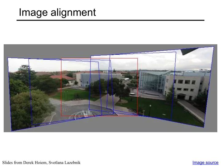
Image alignment Slides from Derek Hoiem, Svetlana Lazebnik Image - - PowerPoint PPT Presentation

Image alignment

Image source Slides from Derek Hoiem, Svetlana Lazebnik

Alignment applications

• A look into the past

Alignment applications

• A look into the past

Alignment applications

• Cool video

Alignment applications

Instance recognition

• T. Weyand and B. Leibe, Visual landmark recognition from Internet photo collections:

A large-scale evaluation, CVIU 2015

Alignment challenges

Small degree of overlap Occlusion, clutter, viewpoint change Intensity changes

Image Alignment

Slide from L. Lazebnik.

Robust feature-based alignment

Slide from L. Lazebnik.

Robust feature-based alignment

• Extract features

Slide from L. Lazebnik.

Robust feature-based alignment

• Extract features
• Compute putative matches

Slide from L. Lazebnik.

Robust feature-based alignment

• Extract features
• Compute putative matches
• Loop:
• Hypothesize transformation T

Slide from L. Lazebnik.

Robust feature-based alignment

• Extract features
• Compute putative matches
• Loop:
• Hypothesize transformation T
• Verify transformation (search for other matches consistent

with T)

Slide from L. Lazebnik.

Generating putative correspondences

?

Slide from L. Lazebnik.

Generating putative correspondences

• Need to compare feature descriptors of local patches

surrounding interest points

( ) ( )

=

?

feature descriptor feature descriptor

?

Slide from L. Lazebnik.

Feature descriptors

• Recall: feature detection and description

Slide from L. Lazebnik.

• Simplest descriptor: vector of raw intensity values
• How to compare two such vectors?
• Sum of squared differences (SSD)

– Not invariant to intensity change

• Normalized correlation

– Invariant to affine intensity change

Feature descriptors

( )

å

• =

i i i

v u

2

) SSD( v u,

÷ ÷ ø ö ç ç è æ

• ÷

÷ ø ö ç ç è æ

• =
• ×
• =

å å å

j j j j i i i

v u v u

2 2

) ( ) ( ) )( ( || || ) ( || || ) ( ) ( v u v u v v v v u u u u v u, r

Slide from L. Lazebnik.

Disadvantage of intensity vectors as descriptors

• Small deformations can affect the matching

score a lot

Slide from L. Lazebnik.

• Descriptor computation:
• Divide patch into 4x4 sub-patches
• Compute histogram of gradient orientations (8 reference

angles) inside each sub-patch

• Resulting descriptor: 4x4x8 = 128 dimensions

Feature descriptors: SIFT

David G. Lowe. "Distinctive image features from scale-invariant keypoints.” IJCV 60 (2), pp. 91-110, 2004.

Slide from L. Lazebnik.

• Descriptor computation:
• Divide patch into 4x4 sub-patches
• Compute histogram of gradient orientations (8 reference

angles) inside each sub-patch

• Resulting descriptor: 4x4x8 = 128 dimensions
• Advantage over raw vectors of pixel values
• Gradients less sensitive to illumination change
• Pooling of gradients over the sub-patches achieves

robustness to small shifts, but still preserves some spatial information

Feature descriptors: SIFT

David G. Lowe. "Distinctive image features from scale-invariant keypoints.” IJCV 60 (2), pp. 91-110, 2004.

Slide from L. Lazebnik.

Feature matching

?

• Generating putative matches: for each patch in one

image, find a short list of patches in the other image that could match it based solely on appearance

Slide from L. Lazebnik.

Problem: Ambiguous putative matches

Source: Y. Furukawa

Rejection of unreliable matches

• How can we tell which putative matches are more reliable?
• Heuristic: compare distance of nearest neighbor to that of

second nearest neighbor

• Ratio of closest distance to second-closest distance will be high

for features that are not distinctive

David G. Lowe. "Distinctive image features from scale-invariant keypoints.” IJCV 60 (2), pp. 91-110, 2004.

Threshold of 0.8 provides good separation

Slide from L. Lazebnik.

RANSAC

• The set of putative matches contains a very high

percentage of outliers RANSAC loop: 1. Randomly select a seed group of matches 2. Compute transformation from seed group 3. Find inliers to this transformation 4. If the number of inliers is sufficiently large, re-compute least-squares estimate of transformation on all of the inliers Keep the transformation with the largest number of inliers

Slide from L. Lazebnik.

Robust feature-based alignment

• Extract features
• Compute putative matches
• Loop:
• Hypothesize transformation T
• Verify transformation (search for other matches consistent

with T)

Slide from L. Lazebnik.

Homography Example

Camera Center

Slide from A. Efros, S. Seitz, D. Hoiem

Common transformations

translation rotation aspect affine perspective

• riginal

Transformed

Slide from A. Efros, S. Seitz, D. Hoiem

Scaling

Scaling a coordinate means multiplying each of its components by a scalar Uniform scaling means this scalar is the same for all components:

´ 2

Slide from A. Efros, S. Seitz, D. Hoiem

Non-uniform scaling: different scalars per component:

Scaling

X ´ 2, Y ´ 0.5

Slide from A. Efros, S. Seitz, D. Hoiem

Scaling

Scaling operation: Or, in matrix form:

by y ax x = = ' ' ú û ù ê ë é ú û ù ê ë é = ú û ù ê ë é y x b a y x ' '

scaling matrix S

Slide from A. Efros, S. Seitz, D. Hoiem

2-D Rotation

q

(x, y) (x’, y’)

x’ = x cos(q) - y sin(q) y’ = x sin(q) + y cos(q)

Slide from A. Efros, S. Seitz, D. Hoiem

2-D Rotation

Polar coordinates… x = r cos (f) y = r sin (f) x’ = r cos (f + q) y’ = r sin (f + q) Trig Identity… x’ = r cos(f) cos(q) – r sin(f) sin(q) y’ = r sin(f) cos(q) + r cos(f) sin(q) Substitute… x’ = x cos(q) - y sin(q) y’ = x sin(q) + y cos(q)

q

(x, y) (x’, y’)

f

Slide from A. Efros, S. Seitz, D. Hoiem

2-D Rotation

This is easy to capture in matrix form: Even though sin(q) and cos(q) are nonlinear functions of q,

• x’ is a linear combination of x and y
• y’ is a linear combination of x and y

What is the inverse transformation?

• Rotation by –q
• For rotation matrices

( ) ( ) ( ) ( )

ú û ù ê ë é ú û ù ê ë é

• =

ú û ù ê ë é y x y x q q q q cos sin sin cos ' '

T

R R =

• 1

R

Slide from A. Efros, S. Seitz, D. Hoiem

Basic 2D transformations

Translate Rotate Shear Scale

ú û ù ê ë é ú û ù ê ë é = ú û ù ê ë é y x y x

y x

1 1 ' ' a a

ú û ù ê ë é ú û ù ê ë é Q Q Q

• Q

= ú û ù ê ë é y x y x cos sin sin cos ' '

ú û ù ê ë é ú û ù ê ë é = ú û ù ê ë é y x s s y x

y x

' '

ú ú ú û ù ê ê ê ë é ú û ù ê ë é = ú û ù ê ë é ¢ ¢ 1 1 1 y x t t y x

y x

ú ú ú û ù ê ê ê ë é ú û ù ê ë é = ú û ù ê ë é ¢ ¢ 1 y x f e d c b a y x

Affine Affine is any combination of translation, scale, rotation, shear

Slide from A. Efros, S. Seitz, D. Hoiem

Affine Transformations

Affine transformations are combinations of

• Linear transformations, and
• Translations

Properties of affine transformations:

• Lines map to lines
• Parallel lines remain parallel
• Ratios are preserved
• Closed under composition

ú ú ú û ù ê ê ê ë é ú û ù ê ë é = ú û ù ê ë é ¢ ¢ 1 y x f e d c b a y x

ú ú ú û ù ê ê ê ë é ú ú ú û ù ê ê ê ë é = ú ú ú û ù ê ê ê ë é 1 1 1 ' ' y x f e d c b a y x

• r

Slide from L. Lazebnik.

Projective Transformations

ú ú û ù ê ê ë é ú ú û ù ê ê ë é = ú ú û ù ê ê ë é w y x i h g f e d c b a w y x ' ' '

Projective transformations are combos of

• Affine transformations, and
• Projective warps

Properties of projective transformations:

• Lines map to lines
• Parallel lines do not necessarily remain parallel
• Ratios are not preserved
• Closed under composition
• Models change of basis
• Projective matrix is defined up to a scale (8 DOF)

Slide from L. Lazebnik.

2D image transformations

Slide from R. Szeliski

Fitting an affine transformation

• Assume we know the correspondences, how do we

get the transformation?

) , (

i i y

x ¢ ¢ ) , (

i i y

x

ú û ù ê ë é + ú û ù ê ë é ú û ù ê ë é = ú û ù ê ë é ¢ ¢

2 1 4 3 2 1

t t y x m m m m y x

i i i i

t Mx x + = ¢

i i

Want to find M, t to minimize

å

=

• ¢

n i i i 1 2

|| || t Mx x

Slide from L. Lazebnik.

Fitting an affine transformation

• Assume we know the correspondences, how do we

get the transformation?

) , (

i i y

x ¢ ¢ ) , (

i i y

x

ú û ù ê ë é + ú û ù ê ë é ú û ù ê ë é = ú û ù ê ë é ¢ ¢

2 1 4 3 2 1

t t y x m m m m y x

i i i i

ú ú ú ú û ù ê ê ê ê ë é ¢ ¢ = ú ú ú ú ú ú ú ú û ù ê ê ê ê ê ê ê ê ë é ú ú ú ú û ù ê ê ê ê ë é ! ! ! !

i i i i i i

y x t t m m m m y x y x

2 1 4 3 2 1

1 1

Slide from L. Lazebnik.

Fitting an affine transformation

• Linear system with six unknowns
• Each match gives us two linearly independent

equations: need at least three to solve for the transformation parameters

ú ú ú ú û ù ê ê ê ê ë é ¢ ¢ = ú ú ú ú ú ú ú ú û ù ê ê ê ê ê ê ê ê ë é ú ú ú ú û ù ê ê ê ê ë é ! ! ! !

i i i i i i

y x t t m m m m y x y x

2 1 4 3 2 1

1 1

Slide from L. Lazebnik.

Fitting a homography

• Recall: homogeneous coordinates

Converting to homogeneous image coordinates Converting from homogeneous image coordinates

Slide from L. Lazebnik.

Fitting a homography

• Recall: homogeneous coordinates
• Equation for homography:

Converting to homogeneous image coordinates Converting from homogeneous image coordinates

ú ú ú û ù ê ê ê ë é ú ú ú û ù ê ê ê ë é = ú ú ú û ù ê ê ê ë é ¢ ¢ 1 1

33 32 31 23 22 21 13 12 11

y x h h h h h h h h h y x l

Slide from L. Lazebnik.

Fitting a homography

• Equation for homography:

i i

x H x = ¢ l

ú ú ú û ù ê ê ê ë é ú ú ú û ù ê ê ê ë é = ú ú ú û ù ê ê ê ë é ¢ ¢ 1 1

33 32 31 23 22 21 13 12 11 i i i i

y x h h h h h h h h h y x l

= ´ ¢

i i

x H x

ú ú ú û ù ê ê ê ë é ¢

• ¢

¢

• ¢

= ú ú ú û ù ê ê ê ë é ´ ú ú ú û ù ê ê ê ë é ¢ ¢

i T i i T i i T i i T i T i T i i T i T i T i i

y x x y y x x h x h x h x h x h x h x h x h x h

3 2 1 1 2 3 1 2 3

1

3 2 1

= ÷ ÷ ÷ ø ö ç ç ç è æ ú ú ú û ù ê ê ê ë é ¢ ¢

• ¢
• ¢
• h

h h x x x x x x

T T i i T i i T i i T T i T i i T i T

x y x y

3 equations,

• nly 2 linearly

independent

Slide from L. Lazebnik.

Fitting a homography

• H has 8 degrees of freedom (9 parameters, but scale is

arbitrary)

• One match gives us two linearly independent equations
• Homogeneous least squares: find h minimizing ||Ah||2
• Eigenvector of ATA corresponding to smallest eigenvalue
• Four matches needed for a minimal solution

3 2 1 1 1 1 1 1 1

= ÷ ÷ ÷ ø ö ç ç ç è æ ú ú ú ú ú ú û ù ê ê ê ê ê ê ë é ¢

• ¢
• ¢
• ¢
• h

h h x x x x x x x x

T n n T T n T n n T n T T T T T T T

x y x y ! ! ! = h A

Slide from L. Lazebnik.

Feature-based alignment: Overview

• Alignment as fitting
• Affine transformations
• Homographies
• Robust alignment
• Descriptor-based feature matching
• RANSAC
• Applications

Slide from L. Lazebnik