Finite-time rupture in thin films driven by non-conservative effects - PowerPoint PPT Presentation

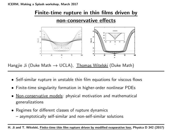
ICERM, Making a Splash workshop, March 2017 Finite-time rupture in thin films driven by non-conservative effects zoom-in 8 8 8 8 0.3 0.2 6 6 6 6 0.1 h ( x, t ) h ( x, t ) h ( x, t ) h ( x, t ) 0 40 45 50 55 60 4 4 4 4 x 2 2 2 2 ǫ ǫ ǫ ǫ 0 0 0 0 0 25 50 75 100 0 0 0 25 25 25 50 50 50 75 75 75 100 100 100 x x x x Hangjie Ji (Duke Math → UCLA), Thomas Witelski (Duke Math) • Self-similar rupture in unstable thin film equations for viscous flows • Finite-time singularity formation in higher-order nonlinear PDEs • Non-conservative models: physical motivation and mathematical generalizations • Regimes for different classes of rupture dynamics – asymptotically self-similar and non-self-similar solutions H. Ji and T. Witelski, Finite-time thin film rupture driven by modified evaporative loss, Physica D 342 (2017)

Classical lubrication models for thin viscous films z z = h ( x, y, t ) x, y Fluid volume: 0 ≤ x, y ≤ L 0 ≤ z ≤ h ( x, y, t ) < H • Navier-Stokes eqns: { � u , p } for viscous incompressible flow • Stokes eqns: Low Reynolds number flow limit, Re → 0 • Slender limit – aspect ratio δ = H/L → 0 : { � u , p } → h ( x, y, t ) • Boundary conditions at z = 0 (substrate) and z = h ( x, y, t ) (free surface) The Reynolds lubrication equation h = h ( x, y, t ) : film height m = m ( h ) : mobility coeff ∂h ∂t = ∇ · ( m ∇ p ) p = p [ h ] : dynamic pressure � J = − m ∇ p : mass flux • m ( h ) ∼ h n : slippage effects, no-slip BC – m ( h ) = h 3 • p = Π( h ) − ∇ 2 h : substrate wettability and surface tension [Oron, Davis, Bankoff 1997, Ockendon and Ockendon 1995, Craster and Matar 2009, ... ]

Representing substrate wettability : The disjoining pressure Fluid-solid intermolecular forces – physico-chemical properties of the solid and fluid. Wetting/non-wetting interactions described by a potential U ( h ) Π( h ) − ∂ 2 h p = Π( h ) ≡ dU ∂h ∂t = ∂ h 3 ∂ � � �� → ∂x 2 dh ∂x ∂x All Π = O ( h − 3 ) → 0 as h → 0 , weak influence for thicker films (a) Hydrophilic materials: Π ∼ − 1 /h 3 Wetting behavior – diffusive spreading of drops ∀ t ≥ 0 (b) Hydrophobic materials: Π ∼ +1 /h 3 Partially wetting – finite spreading of drops (finite support solns) ( Non-wetting – large contact angle, strong repulsion, non-slender regime... ) Dewetting : Instability of uniform coatings of viscous fluids on solid surfaces, Undesirable for many applications (painting, ...). Rich and complex dynamics... [de Gennes 1985, Oron et al 1997, de Gennes et al book 2004, Craster and Matar 2009, Bonn et al 2009]

Simplest model for unstable films with hydrophobic effects ∂x + h 3 ∂ 3 h � � 1 ∂h ∂t = − ∂ h − 1 ∂h ⇒ Π( h ) = = 3 h 3 ∂x 3 ∂x Linear instability of flat films: h ( x, t ) ∼ ¯ h + δ cos( kπx L ) e λt � 1 ¯ � h 3 � λ k = 1 L hk 2 − c k 4 h c = (critical thickness) ¯ h 2 h 2 π c Bifurcation mean-thickness ¯ h  ¯ h < ¯ h c Thin films are unstable  ¯ h > ¯ h c Thicker films stable to infinitesimal perturbations  Bi-stable dynamics for ¯ h > ¯ h c : IC h 0 ( x ) = ( unstable equilibrium ) ± ǫ Relaxation: h → ¯ h or Rupture: h → 0 1 1 � h h h 1 * + 0 0 -1 0 1 -1 0 1 x x [Vrij 1970, Williams & Davis 1982, Laugesen & Pugh 2000]

Van der Waals driven thin film rupture : Finite-time rupture at position x c 0.5 h 0.25 0 1 2 3 x h ( x c , t ) → 0 as t → t c Scaling analysis of rupture in the PDE: let τ = t c − t h = O ( τ 1 / 5 ) → 0 x = O ( τ 2 / 5 ) → 0 as τ → 0 1st-kind self-similar dynamics for formation of a localized singularity, Π → ∞ h ( x, t ) = τ 1 / 5 H ( η ) η = ( x − x c ) /τ 2 / 5 Similarity solution satisfies nonlinear ODE BVP 5 ( H − 2 ηH ′ ) = − ( H − 1 H ′ ) ′ − ( H 3 H ′′′ ) ′ − 1 H ( | η |→ ∞ ) ∼ C | η | 1 / 2 [Zhang & Lister 1999, Witelski & Bernoff 2000] [Barenblatt 1996, Eggers & Fontelos 2009, 2015]

Van der Waals driven thin film rupture : solns of NL similarity ODE BVP 5 ( H − 2 ηH ′ ) = − ( H − 1 H ′ ) ′ − ( H 3 H ′′′ ) ′ H ( | η |→ ∞ ) ∼ C | η | 1 / 2 − 1 4 Using numerical methods, 3 an ∞ -sequence of solns found H 2 k = 1 , 2 , · · · : C k ց 1 [Zhang & Lister 1999, Dallaston et al 2016] 0 -20 -10 0 10 20 η What determines the C k ’s? Exponential asymptotics [Chapman et al 2013] Let H ( η ) = ǫ 2 / 5 φ ( z ) with η = ǫ − 1 / 5 z and ǫ = C 2 → 0 5 ( φ − 2 zφ ′ ) − ( φ − 1 φ ′ ) ′ = ǫ 2 ( φ 3 φ ′′′ ) ′ 1 φ ( | z |→ ∞ ) ∼ z 1 / 2 Analysis of Stokes phenomena from singularities of φ 0 ( z ) in the complex plane 3 0 0 4 8

Continuation after rupture • Solns with Π = h − 3 exist only up to first rupture, 0 ≤ t < t c . • To continue solns to later times, must regularize the singularity and establish a uniform lower bound on h . • Can be accomplished via a modified Π( h ) with balancing conjoining/disjoining effects [Schwartz et al, Oron et al, ...] 1 � ǫ � 3 � Π( h ) = 1 1 − ǫ Π( h ) � ǫ h h 0 0 ǫ h – h ( x, t ) ≥ h min = O ( ǫ ) > 0 (“precursor layer”) – Ensures global existence of solns ∀ t ≥ 0 [Bertozzi, Gr¨ un et al 2001] – Widely-used, physically-motivated regularization • Most studies of singularity formation and rupture in thin films are in the mass-conserving (non-volatile liquid) case • Can lower-order non-conservative effects (e.g. evaporation) cause dramatic differences in the PDE dynamics?

Some non-conservative fourth-order PDE models Π( h ) − ∂ 2 h ∂h ∂t = ∂ ∂ � � �� h n − J ∂x 2 ∂x ∂x [Burelbach et al 1998, Oron et al 2001] ( n = 3 , full Π , E 0 ≶ 0 , K 0 > 0) • γ = 0 : nucleation E 0 J ( h ) = 8 h + K 0 6 h ( x, t ) [Ajaev & Homsy 2001] ( n = 3 , Π = − 1 /h 3 , δ > 0) 4 • 2 J ( h ) = E 0 − δ ( h xx + h − 3 ) ǫ 0 0 25 50 75 100 x h + K 0 γ = − 1 : condensation [Laugesen & Pugh 2000] ( n, Π = h m ) • 8 6 h ( x, t ) J ( h ) = λh 4 2 [Galaktionov 2010] ( n, Π = 0) • ǫ 0 0 25 50 75 100 x J ( h ) = λh ρ 8 [Lindsay et al 2014+] MEMS ( n = 0 , Π = h ) • 6 h ( x, t ) J ( h ) = λ 1 − ǫ � � 4 h 2 h 2 ǫ 0 • Solid films, math biology, ... 0 25 50 75 100 x If | J | is small, yields a separation of timescales in dynamics...

Rupture in a generalized non-conservative Reynolds equation � 1 h 4 + ∂ 2 h ∂h ∂t = ∂ h n ∂p p � � � + p = − h m ∂x 2 ∂x ∂x • Pressure: surface tension and dominant hydrophilic term for Π( h ) for h → 0 (should be stable and prevent rupture) • Non-conservative flux: inspired by Ajaev’s isothermal form, but with opposite sign (destabilizing). Params for physical form of evaporation are stabilizing. • Generalized mobility coefficients h n , h m : inspired by [Bertozzi and Pugh 2000] – they studied finite-time blow-up ( h → ∞ ) in a long-wave unstable eqn h t = − ( h n h xxx ) x − ( h m h x ) x Destabilizing 2nd order term vs. regularizing 4th order term Helpful for tracing/separating competing influences • Here: explore if some form of lower order non-conservative effects can overcome conservative terms and drive finite-time free surface rupture. Obtain a bifurcation diagram for dynamics with ( n, m ) .

Global properties : conservative vs. non-conservative effects � 1 h 4 + ∂ 2 h ∂h ∂t = ∂ h n ∂p p � � � + p = − h m ∂x 2 ∂x ∂x � L • Evolution of fluid mass, M = h dx 0 � L � L � L h 2 d M p Π( h ) x = h m dx = m h m +1 dx + dx h m dt 0 0 0 � L � 2 � ∂h Π( h ) = dU 1 • Evolution of energy, E = + U ( h ) dx 2 ∂x dh 0 � L � L � 2 p 2 d E � ∂p h n dt = − dx + h m dx ∂x 0 0 Not a monotone dissipating Lyapunov functional for this model (unlike the non-conservative/stabilizing [physical] case) • Use local properties at h min ( t ) = h ( x c , t ) = min x h ( x, t ) to characterize the dynamics { ∂ xx h ( x c , t ) , ∂ t h ( x c , t ) } [U. Thiele, Thin film evolution from evaporating ... to epitaxial growth, J. Phys. Condens. Matter 2010]

h ( t ) + δe ikx e σ ( t ) + O ( δ 2 ) 1. Linear stability : perturbed flat films h ( x, t ) = ¯ � 1 � 1 h 4 + ∂ 2 h h 4 + ∂ 2 h � �� � ∂h ∂t = − ∂ h n ∂ 1 − ∂x ∂x ∂x 2 h m ∂x 2 d ¯ h dt = − ¯ h − (4+ m ) O (1) : dσ h − m + ( m + 4)¯ h n + 4 k 2 ¯ � h − ( m +5) � � h n − 5 � k 2 ¯ k 4 ¯ − O ( δ ) : dt = Flat film extinction ¯ h ( t ) → 0 : finite time ( m > − 5) vs. infinite time (exp/alg) dσ Growth of spatial perturbations: dt > 0 if m > − 4 and m + n > 0 � 4 k 2 ¯ � h − ( m +4) → 0  h m + n ¯ h xx ( x c , t ) ∼ C exp m + n < 0  m + n h − ( m +4) → ∞ h xx ( x c , t ) ∼ C ¯ m + n > 0  For m near m ≥ − 4 perturbations grow slowly vs d ¯ h dt before eventual transition 1 10 35 10 30 10 25 0.1 10 20 ( B ) h xx ( x c ) h ( x, t ) 10 15 10 10 0.01 10 5 1 ( C ) 0.001 10 − 5 0 0.2 0.4 0.6 0.8 1 0.001 0.01 0.1 h ( x c ) x