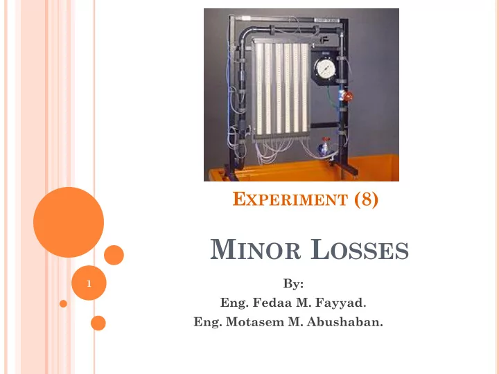
Figure 2 : Schematic drawing of the energy-loss apparatus Figure 3 : - - PowerPoint PPT Presentation

EXPERIMENT (8)

MINOR LOSSES

By:

• Eng. Fedaa M. Fayyad.
• Eng. Motasem M. Abushaban.

1

PURPOSE

 To determine the loss factors for flow through a range of

pipe fittings including bends, a contraction, an enlargement and a gate-valve.

2

APPARATUS

3

Energy Losses in Bends and Fittings Apparatus: It consists of:

• 1. Sudden Enlargement
• 2. Sudden Contraction
• 3. Long Bend
• 4. Short Bend
• 5. Elbow Bend
• 6. Mitre Bend
• 7. Gate Valve

Figure 1: Minor losses apparatus

4

Figure 2 : Schematic drawing of the energy-loss apparatus

5

Figure 3 : Minor Losses Apparatus with hydraulic bench

6

THEORY

g p 

g v 2

2

The energy balance between two points in a pipe can be described by the Bernoulli equation, given by Where:

L

h g V z p g V z p       2 2

2 2 2 2 2 1 1 1

 

Static head or Pressure head Dynamic head or Velocity head Potential head or Elevation head

Z Z g p  

Piezometric head

hl

Head loss

7

THEORY

Head loss, hL, includes

• Major Losses: Sum of pipe friction losses hf
• Minor Losses: hm





 

n 1 i i f L

h h h



Major losses in pipe flows are the result of friction between the fluid and the pipe walls and internal friction between fluid particles. Pipe friction losses are assumed to be negligible in this experiment.

8

THEORY

Head loss, hL, includes

• Sum of pipe friction losses hf
• All minor losses hm





 

n 1 i i f L

h h h



Minor losses occur at any location in a pipe system where streamlines are not straight, such as at pipe junctions, bends, valves, contractions, expansions, and reservoir inlets and outlets. (Any change in the direction of flow or the value of velocity make minor losses)

9

THEORY

 

            g V g V h h hm 2 2 2 1

2 2 2 1

L

h g V z p g V z p       2 2

2 2 2 2 2 1 1 1

 

L

h g V h g V h     2 2 2 1

2 2 2 1

MINOR HEAD LOSSES

 For all bends the diameter does not change, then  For enlargement & contraction, there is a change in the diameter so  Note (h1 - h2) will be negative for the enlargement and

will be negative for the contraction.

10

g v g v 2 / 2 /

2 2 2 1



2 1

h h hm  

 

            g V g V h h hm 2 2 2 1

2 2 2 1

g v g v 2 / 2 /

2 2 2 1



MINOR HEAD LOSSES

 For the gate valve experiment, pressure difference before and

after gate is measured directly using a pressure gauge. This can then be converted to an equivalent head loss using the equation: 1 bar = 10.2 m water

11

LOSS COEFFICIENT

The energy loss which occurs in a pipe fitting (so- called secondary loss) is commonly expressed in terms of a head loss (h, meters) in the form:

12

g V K hm 2

2



LOSS COEFFICIENT

Where K = the loss coefficient and v = mean velocity of flow into the fitting,

For the expansion and contraction, the v used is the velocity of the fluid in the smaller-diameter pipe.

Because of the complexity of flow in many fittings, K is usually determined by experiment. For the pipe fitting experiment, the head loss is calculated from two manometer readings, taken before and after each fitting, and K is then determined as:

13

         g V h K

m

2 /

2

PROCEDURE

 It is not possible to make measurements on all fittings simultaneously

and, therefore, it is necessary to run two separate tests.

PART (A)

1.

Set up the losses apparatus on the hydraulic bench so that its base is horizontal by adjusting the feet on the base plate if necessary. (this is necessary for accurate height measurements from the manometers). Connect the test rig inlet to the bench flow supply and run the outlet extension tube to the volumetric tank and secure it in place.

2.

Fully open the gate valve and the outlet flow control valve at the right hand end of the apparatus.

14

15 3.

Close the bench flow control valve then start the service pump.

4.

Gradually open the bench flow control valve and allow the pipework to fill with water until all air has been expelled from the pipework.

5.

In order to bleed air from pressure tapping points and the manometers close both the bench valve and the test rig flow control valve and open the air bleed screw and remove the cap from the adjacent air valve. Connect a length of small bore tubing from the air valve to the volumetric tank. Now, open the bench valve and allow flow through the manometers to purge all air from them; then, tighten the air bleed screw and partly open both the bench valve and the test rig flow control valve.

6.

Next, open the air bleed screw slightly to allow air to enter the top of the manometers, re-tighten the screw when the manometer levels reach a convenient height.

16

7.

If the levels in the manometer are too high then the hand pump can be used to pressurise the top manifold. All levels will decrease simultaneously but retain the appropriate differentials.

8.

If the levels are too low then the hand pump should be disconnected and the air bleed screw opened briefly to reduce the pressure in the top manifold. Alternatively the outlet flow control valve can be closed to raise the static pressure in the system which will raise all levels simultaneously.

9.

If the level in any manometer tube is allowed to drop too low then air will enter the bottom manifold. If the level in any manometer tube is too high then water will enter the top manifold and flow into adjacent tubes.

17

7.

Adjust the flow from the bench control valve and, at a given flow rate, take height readings from all of the manometers after the levels have steadied. In order to determine the volume flow rate, you should carry out a timed volume collection using the volumetric tank. This is achieved by closing the ball valve and measuring (with a stopwatch) time taken to accumulate a known volume of fluid in the tank, which is read from the sight glass. You should collect fluid for at least one minute to minimize timing errors. ( note: valve should be kept fully open.)

8.

Repeat this procedure to give a total of at least five sets of measurements over a flow range from approximately 8 - 17 liters per minute.

 PART (B)

10.

Clamp off the connecting tubes to the mitre bend pressure tappings (to prevent air being drawn into the system).

11.

Start with the gate valve closed and open fully both the bench valve and the lest rig flow control valve.

12.

• pen the gate valve by approximately 50% of one turn (after taking up

any backlash).

13.

For each of at least 5 flow rates, measure pressure drop across the valve from the pressure gauge; adjust the flow rate by use of the test rig flow control valve. Once measurements have started, do not adjust the gale

• valve. Determine the volume flow rate by timed collection.

14.

Repeat this procedure for the gate valve opened by approximately 70%

• f one turn and then approximately 80% of one turn.

18

DATA & RESULTS

19

The following dimensions from the equipment are used in the appropriate calculations:

• Internal diameter of pipe: d = 0.0183 m
• Internal diameter of pipe at enlargement outlet and contraction inlet : d = 0.0240 m

Table 1. Raw Data for All Fittings Except Gate Valve

Case No. I II III IV V Volume (L) Time (sec) Piezometer Readings (mm) Enlargement 1 2 Contraction 3 4 Long Bend 5 6 Short Bend 7 8 Elbow 9 10 Mitre Bend 11 12

20 Table 2. Raw Data for Gate Valve Case No. I II III IV V 50% Opened Volume (L) Time (sec) Gauge Reading (bar) Red (upstream) Black (downstre am) 70% Opened Volume (L) Time (sec) Gauge Reading (bar) Red (upstream) Black (downstre am) 80% Opened Volume (L) Time (sec) Gauge Reading (bar) Red (upstream) Black (downstre am)

21

CALCULATIONS: FOR PART A

Table 3. Minor Head Losses of All Fittings Except Gate Valve Case No. I II III IV V Q (m3/sec) V (m/s) V2/2g (m) Minor Head Losses (m) Enlargement Δh Δh +V1

2/2g-

V2

2/2g

Contraction Δh Δh +V1

2/2g-

V2

2/2g

Long Bend Short Bend Elbow Mitre Bend

22

• 1. Prepare plots that show the effect of dynamic head (v2/2g) on

minor head loss (hm).

0.1 0.2 0.3 0.4 0.5 0.6 0.7 0.8 0.9 1 0.2 0.4 0.6 0.8 1 head loss (∆h) - m dynamic head (v2/2g) - m

Head loss against dynamic head

Mitre Bend elbow short Bend Enlargement long Bend Contraction

23 Table 4. Loss Coefficients for All Fittings Except Gate Valve Case No. I II III IV V Q (m3/sec) V (m/s) V2/2g (m) Loss Coefficients Enlargement Contraction Long Bend Short Bend Elbow Mitre Bend

24

• 2. Prepare plots that show the effect of flow rate (Q) on loss coefficients (K).

0.1 0.2 0.3 0.4 0.5 0.6 0.7 0.8 0.9 1 0.2 0.4 0.6 0.8 1

loss Coefficients (K) flow rate (Q) - m3/s

Effect of flow rate on loss coefficients

Mitre Bend elbow short Bend Enlargement long Bend Contraction

25 Table 5. Equivalent Minor Head Loss and Loss Coefficient for Gate Valve

Case No. I II III IV V 50% Opened Q (m3/sec) V (m/sec) V2/2g (m) Minor Head Loss (m) Loss Coefficient 70% Opened Q (m3/sec) V (m/sec) V2/2g (m) Minor Head Loss (m) Loss Coefficient 80% Opened Q (m3/sec) V (m/sec) V2/2g (m) Minor Head Loss (m) Loss Coefficient

FOR PART B

26

• 1. Prepare plots that show the effect of dynamic head (v2/2g) on

head loss (hm).

0.1 0.2 0.3 0.4 0.5 0.6 0.7 0.8 0.9 1 0.2 0.4 0.6 0.8 1 head loss (∆h) - m dynamic head (v2/2g) - m

Head loss against dynamic head

50% Opened 70% Opened 80% Opened

27

• 2. Prepare plots that show the effect of flow rate (Q) on loss coefficients (K).

0.1 0.2 0.3 0.4 0.5 0.6 0.7 0.8 0.9 1 0.2 0.4 0.6 0.8 1 loss Coefficients (K) flow rate (Q) - m3/s

Effect of flow rate on loss coefficients

50% Opened 70% Opened 80% Opened

28

QUESTIONS