Exploiting Reductions Given an efficient algorithm for a problem A - PowerPoint PPT Presentation

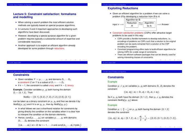
T–79.4201 Search Problems and Algorithms T–79.4201 Search Problems and Algorithms Exploiting Reductions ◮ Given an efficient algorithm for a problem A we can solve a Lecture 5: Constraint satisfaction: formalisms problem B by developing a reduction from B to A . and modelling Algorithm for B: ◮ When solving a search problem the most efficient solution R ( x ) Reduction Algorithm input x = ⇒ = ⇒ = ⇒ Answer R methods are typically based on special purpose algorithms. for A ◮ In Lectures 3 and 4 important approaches to developing such algorithms have been discussed. ◮ Constraint satisfaction problems (CSPs) offer attractive target ◮ However, developing a special purpose algorithm for a given problems to be used in this way: ◮ CSPs provide a flexible framework to develop reductions, i.e., problem requires typically a substantial amount of expertise and encodings of problems as CSPs such that a solution to the original considerable resources. problem can be easily extracted from a solution of the CSP ◮ Another approach is to exploit an efficient algorithm already encoding the problem. developed for some problem through reductions. ◮ Constraint programming offers tools to build efficient algorithms for solving CSPs for a wide range of constraints. ◮ There are efficient software packages that can be directly used for solving interesting classes of constraints. I.N. & P .O. Autumn 2007 1 I.N. & P .O. Autumn 2007 2 T–79.4201 Search Problems and Algorithms T–79.4201 Search Problems and Algorithms Constraints Constraints ◮ Given variables Y := y 1 ,..., y k and domains D 1 ,... D k , a constraint C on Y is a subset of D 1 ×···× D k . Example ◮ If k = 1, the constraint is called unary and if k = 2, binary. Condition y 1 � = y 2 on variables y 1 , y 2 with domains D 1 , D 2 denotes the Example. Consider variables y 1 , y 2 both having the domain constraint { ( d 1 , d 2 ) | d 1 ∈ D 1 , d 2 ∈ D 2 , d 1 � = d 2 } . D i = { 0 , 1 , 2 } . Then NotEq = { ( 0 , 1 ) , ( 0 , 2 ) , ( 1 , 0 ) , ( 1 , 2 ) , ( 2 , 0 ) , ( 2 , 1 ) } So if y 1 , y 2 both have the domain { 0 , 1 , 2 } , then y 1 � = y 2 denotes the constraint NotEq ( y 1 , y 2 ) above. can be taken as a binary constraint on y 1 , y 2 and then we denote it by NotEq ( y 1 , y 2 ) and if it is on y 2 , y 1 , then by NotEq ( y 2 , y 1 ) . Example ◮ In what follows we use a shorthand notation for constraints by Condition y 1 ≤ y 2 4 on y 1 , y 2 both having the domain { 0 , 1 , 2 } 2 + 1 giving directly the condition on the variables when it is clear how denotes the constraint to interpret the condition on the domain elements. { ( d 1 , d 2 ) | d 1 , d 2 ∈ { 0 , 1 , 2 } , d 1 ≤ d 2 2 + 1 ◮ Hence, cond ( y 1 ,..., y k ) on variables y 1 ,..., y k with domains 4 } = { ( 0 , 0 ) , ( 0 , 1 ) , ( 0 , 2 ) , ( 1 , 2 ) } . D 1 ,... D k denotes the constraint { ( d 1 ,..., d k ) | d i ∈ D i for i = 1 ,..., k and cond ( d 1 ,..., d k ) holds } I.N. & P .O. Autumn 2007 3 I.N. & P .O. Autumn 2007 4

T–79.4201 Search Problems and Algorithms T–79.4201 Search Problems and Algorithms CSPs II Constraint Satisfaction Problems (CSPs) ◮ For a CSP � C ; x 1 ∈ D 1 ,..., x n ∈ D n � a potential solution is given ◮ Given variables x 1 ,..., x n and domains D 1 ,... D n , by a value assignment which a mapping T from { x 1 ,..., x n } to D 1 ∪···∪ D n such that for each variable x i , T ( x i ) ∈ D i . a constraint satisfaction problem (CSP): ◮ A value assignment T satisfies a constraint C on variables � C ; x 1 ∈ D 1 ,..., x n ∈ D n � x i 1 ,..., x i m if ( T ( x i 1 ) ,..., T ( x i m )) ∈ C . ◮ Example. A value assignment T = { x 1 �→ 1 , x 2 �→ 2 ,..., x n �→ n } where C is a set of constraints each on a subsequence of satisfies the constraint NotEq on x 1 , x 2 because x 1 ,..., x n . ( T ( x 1 ) , T ( x 2 )) = ( 1 , 2 ) ∈ NotEq but T ′ = { x 1 �→ 1 , x 2 �→ 1 ,..., x n �→ 1 } does not as Example ( T ′ ( x 1 ) , T ′ ( x 2 )) = ( 1 , 1 ) �∈ NotEq . �{ NotEq ( x 1 , x 2 ) , NotEq ( x 1 , x 3 ) , NotEq ( x 2 , x 3 ) } , ◮ A solution to a CSP � C , x 1 ∈ D 1 ,..., x n ∈ D n � is a value x 1 ∈ { 0 , 1 , 2 } , x 2 ∈ { 0 , 1 , 2 } , x 3 ∈ { 0 , 1 , 2 }� assignment that satisfies every constraint C ∈ C . Example. Consider a CSP is a CSP . We often use shorthands for the constrains and write �{ x 1 � = x 2 , x 1 � = x 3 , x 2 � = x 3 } , x 1 ∈ { 0 , 1 , 2 } , x 2 ∈ { 0 , 1 , 2 } , x 3 ∈ { 0 , 1 , 2 }� The assignment { x 1 �→ 0 , x 2 �→ 1 , x 3 �→ 2 } is a solution to the CSP as �{ x 1 � = x 2 , x 1 � = x 3 , x 2 � = x 3 } , x 1 ∈ { 0 , 1 , 2 } , x 2 ∈ { 0 , 1 , 2 } , x 3 ∈ { 0 , 1 , 2 }� it satisfies all the constraints but { x 1 �→ 0 , x 2 �→ 1 , x 3 �→ 1 } is not as it does not satisfy the constraint x 2 � = x 3 ( NotEq ( x 2 , x 3 ) ). I.N. & P .O. Autumn 2007 5 I.N. & P .O. Autumn 2007 6 T–79.4201 Search Problems and Algorithms T–79.4201 Search Problems and Algorithms Example: SEND + MORE = MONEY ◮ Replace each letter by a different digit so that Example: Graph Coloring Problem SEND 9567 Given a graph G , the coloring problem can be encoded as a CSP as + MORE + 1085 follows. MONEY 10652 ◮ For each node v i in the graph introduce a variable V i with the is a correct sum. The unique solution. domain { 1 ,..., n } where n is the number of available colors. ◮ Variables: S, E, N, D, M, O, R, Y ◮ For each edge ( v i , v j ) in the graph introduce a constraint V i � = V j . ◮ Domains: [1..9] for S, M and [0..9] for E, N, D, O, R, Y ◮ Constraints: ◮ This is a reduction of the coloring problem to a CSP because the 1000 · S + 100 · E + 10 · N + D solutions to the CSP correspond exactly to the solutions of the + 1000 · M + 100 · O + 10 · R + E coloring problem: a value assignment { V 1 �→ t 1 ,..., V n �→ t n } satisfying all the = 10000 · M + 1000 · O + 100 · N + 10 · E + Y constraints gives a valid coloring of the graph where node v i is x � = y for every pair of variables x , y in {S, E, N, D, M, O, R, Y}. colored with color t i . ◮ It is easy to check that the value assignment { S �→ 9 , E �→ 5 , N �→ 6 , D �→ 7 , M �→ 1 , O �→ 0 , R �→ 8 , Y �→ 2 } satisfies the constraints, i.e., is a solution to the problem. I.N. & P .O. Autumn 2007 7 I.N. & P .O. Autumn 2007 8

T–79.4201 Search Problems and Algorithms T–79.4201 Search Problems and Algorithms Constrained Optimization Problems N Queens ◮ Given: a CSP P := � C ; x 1 ∈ D 1 ,..., x n ∈ D n � and a function obj Problem: Place n queens on a n × n chess board so that they do not which maps solutions of the CSP to real numbers. attack each other. ◮ ( P , obj ) is a constrained optimization problem (COP) where the task is to find a solution T to P for which the value obj ( T ) is ◮ Variables: x 1 ,..., x n ( x i gives the position of the queen on ith optimal (minimal/maximal). column) ◮ Domains: [1..n] for each x i , i = 1 ,..., n ◮ Example. KNAPSACK: a knapsack of a fixed volume and n objects, each with a volume and a value. Find a collection of ◮ Constraints: for i ∈ [ 1 .. n − 1 ] and j ∈ [ i + 1 .. n ] : these objects with maximal total value that fits in the knapsack. (i) x i � = x j (rows) (ii) x i − x j � = i − j (SW-NE diagonals) ◮ Representation as a COP: Given: knapsack volume v and n objects with volumes a 1 ,..., a n (iii) x i − x j � = j − i (NW-SE diagonals) and values b 1 ,..., b n . ◮ When n = 10, the value assignment { x 1 �→ 3 , x 2 �→ 10 , x 3 �→ Variables: x 1 ,..., x n 7 , x 4 �→ 4 , x 5 �→ 1 , x 6 �→ 5 , x 7 �→ 2 , x 8 �→ 9 , x 9 �→ 6 , x 10 �→ 8 } gives Domains: { 0 , 1 } a solution to the problem. Constraint: ∑ n i = 1 a i · x i ≤ v , Objective function: ∑ n i = 1 b i · x i . I.N. & P .O. Autumn 2007 9 I.N. & P .O. Autumn 2007 10 T–79.4201 Search Problems and Algorithms T–79.4201 Search Problems and Algorithms Solving CSPs Constraints ◮ Constraints have varying computational properties. ◮ For some classes of constraints there are efficient special ◮ In the course we consider more carefully two classes of purpose algorithms (domain specific methods/constraint solvers). constraints: linear constraints and Boolean constraints. Examples ◮ Linear constraints (Lectures 7–9) are an example of a class of ◮ Linear equations constraints which has efficient special purpose algorithms. ◮ Linear programming ◮ Now we consider Boolean constraints as an example of a class ◮ Unification ◮ For others general methods consisting of for which we need to use general methods based on propagation and search. ◮ constraint propagation algorithms and ◮ search methods ◮ However, boolean constraints are interesting because must be used. ◮ highly efficient general purpose methods are available for solving Boolean constraints; ◮ Different encodings of a problem as a CSP utilizing different sets ◮ they provide a flexible framework for encoding (modelling) where it of constraints can have substantial different computational is possible to use combinations of constraints (with efficient properties. support by solution techniques). ◮ However, it is not obvious which encodings lead to the best computational performance. I.N. & P .O. Autumn 2007 11 I.N. & P .O. Autumn 2007 12