Exploiting Reductions Given an efficient algorithm for a problem A - - PowerPoint PPT Presentation

SLIDE 1

T–79.4201 Search Problems and Algorithms

Lecture 5: Constraint satisfaction: formalisms and modelling

◮ When solving a search problem the most efficient solution

methods are typically based on special purpose algorithms.

◮ In Lectures 3 and 4 important approaches to developing such

algorithms have been discussed.

◮ However, developing a special purpose algorithm for a given

problem requires typically a substantial amount of expertise and considerable resources.

◮ Another approach is to exploit an efficient algorithm already

developed for some problem through reductions.

I.N. & P .O. Spring 2006 T–79.4201 Search Problems and Algorithms

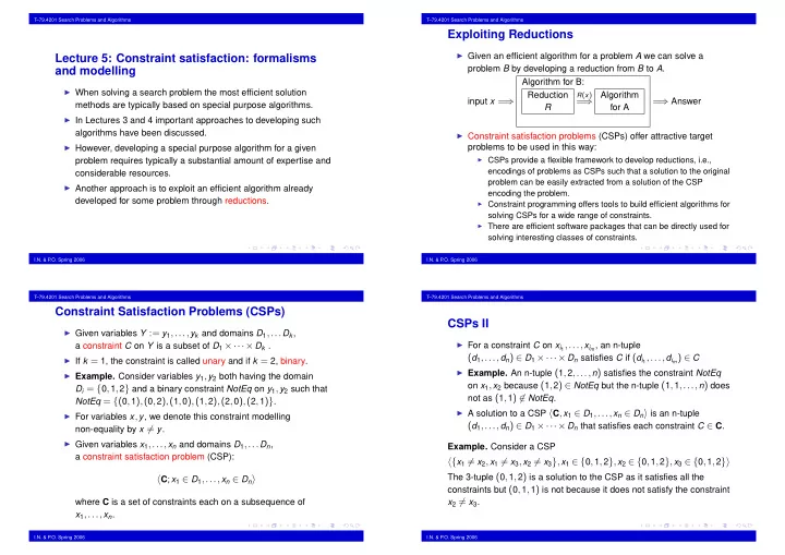
Exploiting Reductions

◮ Given an efficient algorithm for a problem A we can solve a

problem B by developing a reduction from B to A. input x =

⇒

Algorithm for B: Reduction R

R(x)

= ⇒

Algorithm for A

= ⇒ Answer

◮ Constraint satisfaction problems (CSPs) offer attractive target

problems to be used in this way:

◮ CSPs provide a flexible framework to develop reductions, i.e.,

encodings of problems as CSPs such that a solution to the original problem can be easily extracted from a solution of the CSP encoding the problem.

◮ Constraint programming offers tools to build efficient algorithms for

solving CSPs for a wide range of constraints.

◮ There are efficient software packages that can be directly used for

solving interesting classes of constraints.

I.N. & P .O. Spring 2006 T–79.4201 Search Problems and Algorithms

Constraint Satisfaction Problems (CSPs)

◮ Given variables Y := y1,...,yk and domains D1,...Dk,

a constraint C on Y is a subset of D1 ×···× Dk .

◮ If k = 1, the constraint is called unary and if k = 2, binary. ◮ Example. Consider variables y1,y2 both having the domain

Di = {0,1,2} and a binary constraint NotEq on y1,y2 such that NotEq = {(0,1),(0,2),(1,0),(1,2),(2,0),(2,1)}.

◮ For variables x,y, we denote this constraint modelling

non-equality by x = y.

◮ Given variables x1,...,xn and domains D1,...Dn,

a constraint satisfaction problem (CSP):

C;x1 ∈ D1,...,xn ∈ Dn

where C is a set of constraints each on a subsequence of x1,...,xn.

I.N. & P .O. Spring 2006 T–79.4201 Search Problems and Algorithms

CSPs II

◮ For a constraint C on xi1,...,xim, an n-tuple

(d1,...,dn) ∈ D1 ×···× Dn satisfies C if (di1,...,dim) ∈ C

◮ Example. An n-tuple (1,2,...,n) satisfies the constraint NotEq

• n x1,x2 because (1,2) ∈ NotEq but the n-tuple (1,1,...,n) does

not as (1,1) ∈ NotEq.

◮ A solution to a CSP C,x1 ∈ D1,...,xn ∈ Dn is an n-tuple

(d1,...,dn) ∈ D1 ×···× Dn that satisfies each constraint C ∈ C.

• Example. Consider a CSP

{x1 = x2,x1 = x3,x2 = x3},x1 ∈ {0,1,2},x2 ∈ {0,1,2},x3 ∈ {0,1,2}

The 3-tuple (0,1,2) is a solution to the CSP as it satisfies all the constraints but (0,1,1) is not because it does not satisfy the constraint x2 = x3.

I.N. & P .O. Spring 2006

SLIDE 2

T–79.4201 Search Problems and Algorithms

• Example. Coloring problem

Given a graph G, the coloring problem can be encoded as a CSP as follows.

◮ For each node vi in the graph introduce a variable Vi with the

domain {1,...,n} where n is the number of available colors.

◮ For each edge (vi,vj) in the graph introduce a constraint Vi = Vj. ◮ This is a reduction of the coloring problem to a CSP because the

solutions to the CSP correspond exactly to the solutions of the coloring problem: a tuple (t1,...,tn) satisfying all the constraints gives a valid coloring of the graph where node vi is colored with color ti.

I.N. & P .O. Spring 2006 T–79.4201 Search Problems and Algorithms

Example: SEND + MORE = MONEY

◮ Replace each letter by a different digit so that

SEND + MORE MONEY 9567 + 1085 10652 is a correct sum. The unique solution.

◮ Variables: S, E, N, D, M, O, R, Y ◮ Domains: [1..9] for S, M and [0..9] for E, N, D, O, R, Y ◮ Constraints:

1000· S + 100· E + 10· N + D

+1000· M + 100· O + 10· R + E = 10000· M + 1000· O + 100· N + 10· E + Y

x = y for every pair of variables x,y in {S, E, N, D, M, O, R, Y}.

◮ It is easy to check that the tuple (9,5,6,7,1,0,8,2) satisfies the

constraints, i.e., is a solution to the problem.

I.N. & P .O. Spring 2006 T–79.4201 Search Problems and Algorithms

N Queens

Problem: Place n queens on a n × n chess board so that they do not attack each other.

◮ Variables: x1,...,xn (xi gives the position of the queen on ith

column)

◮ Domains: [1..n] ◮ Constraints: for i ∈ [1..n − 1] and j ∈ [i + 1..n]:

(i) xi = xj (rows) (ii) xi − xj = i − j (SW-NE diagonals) (iii) xi − xj = j − i (NW-SE diagonals)

◮ When n = 10, the tuple (3,10,7,4,1,5,2,9,6,8) gives a solution

to the problem.

I.N. & P .O. Spring 2006 T–79.4201 Search Problems and Algorithms

Constrained Optimization Problems

◮ Given: a CSP P := C;x1 ∈ D1,...,xn ∈ Dn and a function

• bj : Sol → R

◮ (P,obj) is a constrained optimization problem (COP) where the

task is to find a solution d to P for which the value obj(d) is

• ptimal.

◮ Example. KNAPSACK: a knapsack of a fixed volume and n

• bjects, each with a volume and a value. Find a collection of

these objects with maximal total value that fits in the knapsack.

◮ Representation as a COP:

Given: knapsack volume v and n objects with volumes a1,...,an and values b1,...,bn. Variables: x1,...,xn Domains: {0,1} Constraint: ∑n

i=1 ai · xi ≤ v,

Objective function: ∑n

i=1 bi · xi.

I.N. & P .O. Spring 2006

SLIDE 3

T–79.4201 Search Problems and Algorithms

Solving CSPs

◮ Constraints have varying computational properties. ◮ For some classes of constraints there are efficient special

purpose algorithms (domain specific methods/constraint solvers). Examples

◮ Linear equations ◮ Linear programming ◮ Unification

◮ For others general methods consisting of

◮ constraint propagation algorithms and ◮ search methods

must be used.

◮ Different encodings of a problem as a CSP utilizing different sets

• f constraints can have substantial different computational

properties.

◮ However, it is not obvious which encodings lead to the best

computational performance.

I.N. & P .O. Spring 2006 T–79.4201 Search Problems and Algorithms

Constraints

◮ In the course we consider more carefully two classes of

constraints: linear constraints and Boolean constraints.

◮ Linear constraints (Lectures 7–9) are an example of a class of

constraints which has efficient special purpose algorithms.

◮ Now we consider Boolean constraints as an example of a class

for which we need to use general methods based on propagation and search.

◮ However, boolean constraints are interesting because

◮ highly efficient general purpose methods are available for solving

Boolean constraints;

◮ they provide a flexible framework for encoding (modelling) where it

is possible to use combinations of constraints (with efficient support by solution techniques).

I.N. & P .O. Spring 2006 T–79.4201 Search Problems and Algorithms

Boolean Constraints

◮ A Boolean constraint C on variables x1,...,xn with the domain

{true,false} can be seen as a Boolean function

fC : {true,false}n −

→ {true,false} such that a tuple (t1,...,tn)

satisfies the constraint C iff fC(t1,...,tn) = true.

◮ Typically such functions are represented as propositional

formulas.

◮ Solution methods for Boolean constraints exploit the structure of

the representation of the constraints as formulas.

I.N. & P .O. Spring 2006 T–79.4201 Search Problems and Algorithms

Propositional formulas

◮ Syntax (what are well-formed propositional formulas):

Boolean variables (atoms) X = {x1,x2,...} Boolean connectives ∨,∧,¬

◮ The set of (propositional) formulas is the smallest set such that all

Boolean variables are formulas and if φ1 and φ2 are formulas, so are ¬φ1, (φ1 ∧φ2), and (φ1 ∨φ2). For example, ((x1 ∨ x2)∧¬x3) is a formula but ((x1 ∨ x2)¬x3) is not.

◮ A formula of the form xi or ¬xi is called a literal where xi is a

Boolean variable.

◮ We employ usual shorthands:

φ1 → φ2: ¬φ1 ∨φ2 φ1 ↔ φ2: (¬φ1 ∨φ2)∧(¬φ2 ∨φ1) φ1 ⊕φ2: (¬φ1 ∧φ2)∨(φ1 ∧¬φ2)

I.N. & P .O. Spring 2006

SLIDE 4

T–79.4201 Search Problems and Algorithms

Semantics

◮ Atomic proposition (Boolean variables) are either true or false

and this induces a truth value for any formula as follows.

◮ A truth assignment T is mapping from a finite subset X ′ ⊂ X to

the set of truth values {true,false}.

◮ Consider a truth assignment T : X ′ −

→ {true,false} which is

appropriate to φ, i.e., X(φ) ⊆ X ′ where X(φ) be the set of Boolean variables appearing in φ.

◮ T |

= φ (T satisfies φ) is defined inductively as follows:

If φ is a variable, then T |

= φ iff T(φ) = true.

If φ = ¬φ1, then T |

= φ iff T | = φ1

If φ = φ1 ∧φ2, then T |

= φ iff T | = φ1 and T | = φ2

If φ = φ1 ∨φ2, then T |

= φ iff T | = φ1 or T | = φ2 Example

Let T(x1) = true, T(x2) = false. Then T |

= x1 ∨ x2 but T | = (x1 ∨¬x2)∧(¬x1 ∧ x2)

I.N. & P .O. Spring 2006 T–79.4201 Search Problems and Algorithms

Representing Boolean Functions

◮ A propositional formula φ with variables x1,...,xn expresses a

n-ary Boolean function f if for any n-tuple of truth values t = (t1,...,tn), f(t) = true if T |

= φ and f(t) = false if T | = φ

where T(xi) = ti, i = 1,...,n.

• Proposition. Any n-ary Boolean function f can be expressed as a

propositional formula φf involving variables x1,...,xn.

◮ The idea: model the rows of the truth

table giving true as a disjunction of conjunctions.

◮ Let F be the set of all n-tuples

t = (t1,...,tn) with f(t) = true. For each t, let Dt be a conjunction of literals xi if ti = true and ¬xi if ti = false.

◮ Let φf = W

t∈F Dt

Note that φf is big in the worst case: Example. x1 x2 f 1 1 1 1 1 1

φf = (¬x1 ∧ x2)∨ (x1 ∧¬x2)

I.N. & P .O. Spring 2006 T–79.4201 Search Problems and Algorithms

Logical Equivalence

Definition

Formulas φ1 and φ2 are equivalent (φ1 ≡ φ2) iff for all truth assignments T appropriate to both of them, T |

= φ1 iff T | = φ2. Example (φ1 ∨φ2) ≡ (φ2 ∨φ1) ((φ1 ∧φ2)∧φ3) ≡ (φ1 ∧(φ2 ∧φ3)) ¬¬φ ≡ φ ((φ1 ∧φ2)∨φ3) ≡ ((φ1 ∨φ3)∧(φ2 ∨φ3)) ¬(φ1 ∧φ2) ≡ (¬φ1 ∨¬φ2) (φ1 ∨φ1) ≡ φ1

◮ Simplified notation:

(((x1 ∨¬x3)∨ x2)∨ x4 ∨(x2 ∨ x5)) is written as

x1 ∨¬x3 ∨ x2 ∨ x4 ∨ x2 ∨ x5

• r

x1 ∨¬x3 ∨ x2 ∨ x4 ∨ x5

◮ Wn

i=1 ϕi stands for ϕ1 ∨···∨ϕn

Vn

i=1 ϕi stands for ϕ1 ∧···∧ϕn

I.N. & P .O. Spring 2006 T–79.4201 Search Problems and Algorithms

Normal Forms

◮ Many solvers for Boolean constraints require that the constraints

are represented in a normal form (typically in conjunctive normal form).

• Proposition. Every propositional formula is equivalent to one in

conjunctive (disjunctive) normal form. CNF: (l11 ∨···∨ l1n1)∧···∧(lm1 ∨···∨ lmnm) DNF: (l11 ∧···∧ l1n1)∨···∨(lm1 ∧···∧ lmnm) where each lij is a literal (Boolean variable or its negation). A disjunction l1 ∨···∨ ln is called a clause. A conjunction l1 ∧···∧ ln is called an implicant.

I.N. & P .O. Spring 2006

SLIDE 5

T–79.4201 Search Problems and Algorithms

Normal Form Transformations

CNF/DNF transformation:

• 1. remove ↔ and →:

α ↔ β ❀ (¬α∨β)∧(¬β∨α)

(1)

α → β ❀ ¬α∨β

(2)

• 2. Push negations in front of Boolean variables:

¬¬α ❀ α

(3)

¬(α∨β) ❀ ¬α∧¬β

(4)

¬(α∧β) ❀ ¬α∨¬β

(5)

• 3. CNF: move ∧ connectives outside ∨ connectives:

α∨(β∧γ) ❀ (α∨β)∧(α∨γ)

(6)

(α∧β)∨γ ❀ (α∨γ)∧(β∨γ)

(7) DNF: move ∨ connectives outside ∧ connectives:

α∧(β∨γ) ❀ (α∧β)∨(α∧γ)

(8)

(α∨β)∧γ ❀ (α∧γ)∨(β∧γ)

(9)

I.N. & P .O. Spring 2006 T–79.4201 Search Problems and Algorithms

Example

Transform (A∨ B) → (B ↔ C) to CNF.

(A∨ B) → (B ↔ C)

(1,2)

¬(A∨ B)∨((¬B ∨ C)∧(¬C ∨ B))

(4)

(¬A∧¬B)∨((¬B ∨ C)∧(¬C ∨ B))

(7)

(¬A∨((¬B ∨ C)∧(¬C ∨ B)))∧(¬B ∨((¬B ∨ C)∧(¬C ∨ B))) (6) ((¬A∨(¬B ∨ C))∧(¬A∨(¬C ∨ B)))∧(¬B ∨((¬B ∨ C)∧(¬C ∨ B))) (6) ((¬A∨(¬B ∨ C))∧(¬A∨(¬C ∨ B)))∧((¬B ∨(¬B ∨ C))∧(¬B ∨(¬C ∨ B)) (¬A∨¬B ∨ C)∧(¬A∨¬C ∨ B)∧(¬B ∨¬B ∨ C)∧(¬B ∨¬C ∨ B)

◮ We can assume that normal forms do not have repeated

clauses/implicants or repeated literals in clauses/implicants (for example (¬B ∨¬B ∨ C) ≡ (¬B ∨ C)).

◮ Normal form can be exponentially bigger than the original formula

in the worst case.

I.N. & P .O. Spring 2006 T–79.4201 Search Problems and Algorithms

Boolean Circuits

◮ Normal forms are often a quite unnatural way of encoding

problems as a propositional formula.

◮ More natural encodings are obtained using Boolean circuits to

represent the required Boolean functions

◮ A Boolean circuit C is a 4-tuple (V,E,s,α) where ◮ (V,E) is an acyclic graph whose

nodes are called gates. The nodes are divided into three categories:

◮ output gates (outdegree 0) ◮ intermediate gates ◮ input gates (indgree 0)

◮ s assigns a Boolean function s(g) to

each intermediate and output gate g

• f appropriate arity corresponding to

the indegree of the gate.

◮ α assigns truth values to some gates.

and

• r

equiv ⊥ v4 v5 v6 v3 v2 v1

I.N. & P .O. Spring 2006 T–79.4201 Search Problems and Algorithms

Boolean Circuits—Semantics

◮ For a circuit a truth assignment T : X(C) −

→ {true,false} gives

a truth assignment to each input gate X(C) of C.

◮ This defines a truth value T(g) for each gate g inductively if the

gates are ordered topologically in a sequence so that no gate appears in the sequence before its input gates (this is always possible because the circuit is acyclic):

◮ If g ∈ X(C), then the truth assignment T(g) gives the truth value. ◮ Otherwise T(g) = f(T(g1),...,T(gn)) where (g1,g), . . . and

(gn,g) are the edges entering g and f is the Boolean function

s(g) associated to g.

I.N. & P .O. Spring 2006

SLIDE 6

T–79.4201 Search Problems and Algorithms

Circuit Satisfiability Problem

◮ An interesting computational (search) problem related to circuits

is the circuit satisfiability problem.

◮ Given a Boolean circuit (V,E,s,α) we say a truth assignment T

satisfies the circuit if it satisfies the constraints α, i.e., for each gate g for which α gives a truth value, α(g) = T(g) holds.

◮ CIRCUIT SAT problem: Given a Boolean circuit find a truth

assignment T that satisfies the circuit.

• Example. Consider the circuit given on

the right with constraints

α(v4) = false and α(v1) = true.

This circuit has a satisfying truth as- signment T(v4) = false,T(v5) = T(v6) = true.

and

• r

equiv ⊥ v4 v5 v6 v3 v2 v1

I.N. & P .O. Spring 2006 T–79.4201 Search Problems and Algorithms

Boolean Circuits vs. Propositional Formulas

◮ For each propositional formulae φ, there is a corresponding

Boolean circuit Cφ such that for any T appropriate for both, T(gφ) = true iff T |

= φ for an output gate gφ of Cφ .

Idea: just introduce a new gate for each subexpression.

(a∨ b)∧(¬a∨ b)∧ (a∨¬b)∧(¬a∨¬b)

• r
• r
• r

and

• r

not not

b a c d f e g h v ◮ For each Boolean circuit C, there is a corresponding formula φC. ◮ Notice that Boolean circuits allow shared subexpressions but

formulas do not.

I.N. & P .O. Spring 2006 T–79.4201 Search Problems and Algorithms

Circuits Compute Boolean Functions

◮ A Boolean circuit with output gate g and variables x1,...,xn

computes an n-ary Boolean function f if for any n-tuple of truth values t = (t1,...,tn), f(t) = T(g) where T(xi) = ti, i = 1,...,n.

◮ Any n-ary Boolean function f can be computed by a Boolean

circuit involving variables x1,...,xn.

◮ Not every Boolean function can be computed using a concise

circuit.

Theorem

For any n ≥ 2 there is an n-ary Boolean function f such that no Boolean circuit with 2n

2n or fewer gates can compute it.

I.N. & P .O. Spring 2006 T–79.4201 Search Problems and Algorithms

Boolean Circuits as Equation Systems

A Boolean circuit can be written as a system of equations.

• r
• r
• r

and

• r

not not

b a c d f e g h v

v = and(e,f,g,h) e = or(a,b) f = or(b,c) g = or(a,d) h = or(c,d) c = not(a) d = not(b)

I.N. & P .O. Spring 2006

SLIDE 7

T–79.4201 Search Problems and Algorithms

Boolean Modelling

◮ Propositional formulas/Boolean circuits offer a natural way of

modelling many interesting Boolean functions.

◮ Example. IF-THEN-ELSE ite(a,b,c) (if a then b else c.).

As a formula: ite(a,b,c) ≡ (a∧ b)∨(¬a∧ c) As a circuit: i = or(i1,i2) i1 = and(a,b) i2 = and(a1,c) a1 = not(a)

◮ Given gates a,b,c, ite(a,b,c) can be thought as a shorthand for

a subcircuit given above.

◮ In the bczchaff tool used in the course ite(a,b,c) is provided as

a primitive gate functions.

I.N. & P .O. Spring 2006 T–79.4201 Search Problems and Algorithms

Example

Binary adder. Given input bits a, b and c compute output bits o2o1 which give the sum of a, b, and c in binary. As a formula:

• 1 ≡ ((a⊕ b)⊕ c)
• 2 ≡ (a∧ b)∨(c ∧(a⊕ b)

As a circuit:

• 1 = xor(x,c)
• 2 = or(l,r)

l = and(a,b) r = and(c,x) x = xor(a,b)

I.N. & P .O. Spring 2006 T–79.4201 Search Problems and Algorithms

Encoding Problems Using Circuits

◮ Circuits can be used to encode problems in a structured way. ◮ Example. Given three bits a,b,c find their values such that

if at least two of them are ones then either a or b is one else a or c is one.

◮ We use IF-THEN-ELSE and adder circuits to encode this as a

CIRCUIT SAT problem as follows: p = ite(o2,x,p1) p1 = or(a,c) % full adder; gate o1 omitted

• 2 = or(l,r)

l = and(a,b) r = and(c,x) x = xor(a,b)

◮ Now each satisfying truth assignment for the circuit with

α(p) = true gives a solution to the problem.

I.N. & P .O. Spring 2006 T–79.4201 Search Problems and Algorithms

• Example. Reachability

Given a graph G = ({1,...,n},E), constructs a circuit R(G) such that R(G) is satisfiable iff there is a path from 1 to n in G.

◮ The gates of R(G) are of the form

gijk with 1 ≤ i,j ≤ n and 0 ≤ k ≤ n hijk with 1 ≤ i,j,k ≤ n

◮ gijk is true: there is a path in G from i to j not using any

intermediate node bigger than k.

◮ hijk is true: there is a path in G from i to j not using any

intermediate node bigger than k but using k.

I.N. & P .O. Spring 2006

SLIDE 8

T–79.4201 Search Problems and Algorithms

Example—cont’d

R(G) is the following circuit:

◮ For k = 0, gijk is an input gate. ◮ For k = 1,2,...,n:

hijk = and(gik(k−1),gkj(k−1)) gijk = or(gij(k−1),hijk)

◮ g1nn is the output gate of R(G). ◮ Constraints α:

For the output gate: α(g1nn) = true For the input gates: α(gij0) = true if i = j or (i,j) is an edge in G else α(gij0) = false.

I.N. & P .O. Spring 2006 T–79.4201 Search Problems and Algorithms

Example—cont’d

◮ Because of the constraints α on input gates there is at most one

possible truth assignment T.

◮ It can be shown by induction on k = 0,1,...,n that in this

assignment the truth values of the gates correspond to their given intuitive readings.

◮ From this it follows:

R(G) is satisfiable iff T(g1nn) = true in the truth assignment iff there is a path from 1 to n in G without any intermediate nodes bigger than n iff there is a path from 1 to n in G.

I.N. & P .O. Spring 2006 T–79.4201 Search Problems and Algorithms

• Example. Reachability with choices

◮ Consider now a more challenging (search problem). ◮ For odd numbered nodes i (but not for 1 and n) there are two

alternative edges either to the node i + 1 or to i − 1 and for the

• ther nodes the edges are given as in G.

◮ Find the set of edges for the odd nodes such that there is a path

from 1 to n.

◮ To solve this problem we can use the circuit R(G) and modify it

for each odd node i as follows:

◮ add a subcircuit xi = xor(gi,i+1,0,gi,i−1,0) and set α(xi) = true; ◮ remove constraints α(gi,i+1,0) = t and α(gi,i−1,0) = t′.

◮ Now the modified R(G) is satisfiable iff there is a set of edges for

the odd nodes such that there is a path from 1 to n.

◮ Moreover, the set of edges is given by the gates gi,i−1,0,gi,i+1,0

true in a satisfying truth assignment.

I.N. & P .O. Spring 2006 T–79.4201 Search Problems and Algorithms

From Circuits to CNF

◮ Translating Boolean Circuits to an equivalent CNF formula can

lead to exponential blow-up in the size of the formula.

◮ Often exact equivalence is not necessary but auxiliary variables

can be used as long as at least satisfiability is preserved.

◮ Then a linear size CNF representation can be obtained using

co-called Tseitin translation where given a Boolean circuit C the corresponding CNF formula is obtained as follows

◮ a new variable is introduced to each gate of the circuit, ◮ the set of clauses in the normal form consist of the gate equation

is written in a clausal form for each intermediate and output gate and the corresponding literal for each gate g with a constraint

α(g) = t.

◮ This transformation preserves satisfiability and even truth

assignments in the following sense: if C is a Boolean circuit and Σ its Tseitin translation, then for every truth assignment T of C there is a satisfying truth assignment T ′ of Σ which agrees with T and vice versa.

I.N. & P .O. Spring 2006

SLIDE 9

T–79.4201 Search Problems and Algorithms

From Circuits to CNF II

Example.

and

• r

equiv ⊥ v4 v5 v6 v3 v2 v1

Gate equations for non-input gates: v1 ↔ (v2 ∧ v3) v2 ↔ (v4 ∨ v5 ∨ v6) v3 ↔ (v5 ↔ v6) In CNF:

(¬v1 ∨ v2)∧(¬v1 ∨ v3)∧(v1 ∨¬v2 ∨¬v3)∧ (v2 ∨¬v4)∧(v2 ∨¬v5)∧(v2 ∨¬v6)∧(¬v2 ∨ v4 ∨ v5 ∨ v6)∧ (v3 ∨v5 ∨v6)∧(v3 ∨¬v5 ∨¬v6)∧(¬v3 ∨v5 ∨¬v6)∧(¬v3 ∨¬v5 ∨v6)∧ (¬v4) (for the constraint α(v4) = false)

I.N. & P .O. Spring 2006