ETNA (Efficiency Transfer for Nuclide Activity measurement) ETNA is - - PowerPoint PPT Presentation

ETNA

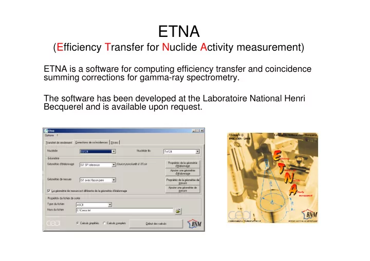
(Efficiency Transfer for Nuclide Activity measurement)

ETNA is a software for computing efficiency transfer and coincidence summing corrections for gamma-ray spectrometry. The software has been developed at the Laboratoire National Henri Becquerel and is available upon request.

ETNA

• Transfer of efficiency

– Semi-empirical method (from a reference efficiency) – Coaxial cylindrical geometry (point. disk. cylinder. Marinelli)

• Coincidence summing corrections

– Knowledge of the efficiency (total and full-energy peak) – Possibility of efficiency transfer – Decay scheme from Nucleide

• Data management

– Decay scheme – Attenuation coefficients

ETNA main window

Recent update (04/11/2010)

Thanks to Dr Aldo FAZIO (ENEA) !

Efficiency transfer principle

) (P (E). = ) P (E, Ω

ε ε

I

Point source moving along the detector axis

) (P (P) ). P (E, = P) (E, Ω Ω

ε ε

(P) (E). = P) (E, Ω

ε ε

I

Solid angle for point source

The geometrical factor should include:

• attenuation in differents absorbing layers (air, window, dead layer. …) : Fatt
• absorption in the detector active volume : Fabs

Using polar coodinates. the solid angle Ω(P) between point P (r, φ, zs) and the detector entrance surface (disc) is: RD is the detector radius.

• +

+ ϕ ⋅ ⋅ ⋅ − ⋅ ϕ ⋅ = Ω

π

• R

2 / 3 2 S 2 2 S

D

z r cos r R 2 R dR R d z 2 ) P (

• δ

⋅ µ − =

• =

m 1 i i i att exp

F

' f f f F

2 1 abs

⋅ + =

( )

D 1 D 1

exp 1 f δ ⋅ µ − − =

( )

D 2 D 2

exp 1 f δ ⋅ µ − − =

( ) ( )

D 1 D

exp ' f δ + ∆ ⋅ µ − =

Solid angle for a cylindrical source

• For a volume source (cylindrical symmetry : radius RS,

thickness HS, vertical position ZS):

• Fatt and F abs must be included in the integration

procedure

• +

+ ϕ ⋅ ⋅ ⋅ − ⋅ ϕ ⋅ ⋅ ⋅ = Ω

+

• π
• S

S S D S

H Z Z R 2 / 3 2 2 2 R S 2 S

h r cos r R 2 R dR R d dr r dh h H R 4

Solid angle for a cylindrical source

V1 V2 V2 S1 S2 V1

RD RS HS HD

If the source diameter is larger than the detector one:

2 1 2 S ) 2 V ( 1 S ) 2 V 1 V (

d d Ω + Ω = Ω + Ω = Ω

• +
• +

+ ϕ ⋅ ⋅ ⋅ − ⋅ ⋅ ⋅ ϕ ⋅ ⋅ ⋅ = Ω

+

• π
• S

S S D S

H Z Z R 2 / 3 2 2 2 abs att R S 2 S 1

h r cos r R 2 R dR R F F d dr r dh h H R 4

( )

• +

+ ⋅ ⋅ ⋅ − ⋅ − ⋅ ⋅ ⋅ ⋅ ⋅ ⋅ = Ω

+

• S

S S D S

H Z Z Z D abs att R s S D

h r r R R dz R r F F d dr r dh H R R

2 / 3 2 2 2 2 2

cos 2 cos 4 ϕ ϕ ϕ

φ

Integration method

• Integration are numerically performed

using the Gauss-Legendre method:

• Point sources, discs, cylinders and

Marinelli (along the detector axis) are considered.

xi and wi = roots and weights of Legendre polynomials

( )

• =

− =

b a n 1 i i i

) x ( f w 2 a b dx ) x ( f

( ) ( )

2 a b x 2 a b ) x ( f

i i

+ + − =

Input of data

• Requires

– Detector parameters – Source parameters

• Container
• Matrix

– Geometry conditions (source-to-detector distance, screen) – Reference efficiency

• Recorded in the « user » database

Efficiency transfer window

Input of geometry parameters

Input of detector parameters

Input of source parameters

• Source : type and characteristics (container and material)

Input of calibration efficiencies

Manual input Function (APOCOPE or APOLOG) File import

Efficiency transfer results

Coincidence summing

Calculation principle

• ETNA uses a numerical method, according

to Andreev, Mc Callum principle:

2 T 12 1

P 1 1 C ε ⋅ − =

1 T 21 2

P 1 1 C ε ⋅ − =

X Y Z A β β β β- γ1

2

γ

3

γ Z + 1

• ⋅

⋅ ⋅ + =

12 3 P 2 P 1 P 3 1 3

P I I 1 1 C ε ε ε

γ γ

P12 : probability for emitting γ2 simultaneaously with γ1 εPi : FEP efficiency for energy Ei εTi : Total efficiency for energy Ei

Calculation principle (2)

• Double coincidences
• Coincidences with K X-rays (electron capture or

internal conversion) are computed

• Correction for K-X-rays (from gamma or X rays)

are computed

• Beta+ emitting nuclides are considered

(modification of the decay scheme)

• No angular correlation

ETNA – Input data

ETNA requires:

• 1. Decay scheme (Nucleide database)
• 2. FEP and total efficiency for at least one

source-to-detector geometry («calibration geometry » recorded in the « user » database)

ETNA – Coincidence tab

From Nucleide

Calibration geometry window

Efficiency calibration

Coincidence correction results

• dimanche 22 février 2009
• ETNA __________________________________Version 5.5 Rev 51
• Filename :C:\Documents and Settings\ML118236\Bureau\Workshop_ICRM\Presentations\ETNA\test_ETNA
• dimanche 22 février 2009
• Processing identification : Coincidence summing correction (simplified computing)
• Nuclide :Ba133
• Daughter nuclide :Cs133
• Half-life threshold :0.000001 s
• Calibration geometry : G1 SP reference (Source ponctuelle à 10 cm)
• Calibration source :Source ponctuelle
• Calibration source - detector distance :100 mm
• Calibration absorber :None
• Calibration absorber - detector distance :0 mm
• Measurement geometry :Calibration geometry
• Detector :G1 - pièce 6A
• Results :
• Error codes : 0 0
• X-ray correction : 01.015880
• Starting

Arrival Energy Gamma-gamma Gamma-X Total

• level

level (keV) correction correction correction

• 004 003 00053.162 01.013962 01.010219 01.024324
• 002 001 00079.614 01.015207 01.012325 01.027720
• 001 000 00080.998 01.011478 01.007984 01.019554
• 002 000 00160.612 00.993490 01.007235 01.000678
• 003 002 00223.237 01.009461 01.019791 01.029439
• 004 002 00276.399 01.008560 01.015827 01.024522
• 003 001 00302.851 01.005028 01.015414 01.020519
• 004 001 00356.013 01.003565 01.011468 01.015074
• 003 000 00383.849 00.991597 01.010308 01.001818
• :
• CEA\LNHB ______________________________________ BNM

Calculation with efficiency transfer

Data update

Decay scheme data Attenuation coefficients Nucléide: import of updated data (only for LNHB !)

Data update

• Attenuation

coefficients

• Manual input
• File import

(XCOM or ASCII)

Attenuation coefficients

Import file from XCOM

Experimental validation (1)

• Efficiency transfer: point source from 1 to 25 cm from detector window

137Cs et 57Co (with Al screen): no coincidences

• Reference peak area: 10 cm

137Cs (662 keV) 57Co (122 keV)

Source-to- detector distance Experiment al peak relative area ETNA Ratio ETNA/Expe rimental Experiment al peak relative area ETNA Ratio ETNA/Expe rimental 25 cm 0.206 (1) 0.206 (5) 0.998 0.188 (1) 0.188 (4) 0.997 20 cm 0.308 (1) 0.308 (6) 1.000 0.287 (1) 0.286 (6) 0.996 15 cm 0.510 (1) 0.509 (10) 1.000 0.486 (2) 0.486 (11) 0.998 8 cm 1.423 (3) 1.420 (36) 0.998 1.458 (5) 1.46 (40) 1.001 6 cm 2.172 (5) 2.18 (7) 1.006 2.321 (7) 2.32 (8) 1.000 5 cm 2.785 (6) 2.82 (9) 1.013 3.065 (10) 3.06 (11) 0.998 4 cm 3.717 (8) 3.75 (14) 1.008 4.187 (13) 4.18 (18) 0.999 3 cm 5.159 (12) 5.21 (24) 1.010 6.026 (19) 6.00 (30) 0.996 2 cm 7.678 (17) 7.73 (43) 1.006 9.276 (29) 9.19 (55) 0.991 1 cm 12.40 (3) 12.4 (10) 1.000 15.36 (5) 15.1 (13) 0.981

Maximum relative standard uncertainties: (parameters uncertainties) 2.2 % at 15 cm – 2.8 % at 8 cm – 3.7 % at 5 cm – 5 % at 3 cm - 8.5 % at 1 cm

• EUROMET Exercice
• Comparison of software used to compute transfer

efficiency

• Experimental calibration for 3 volume sources
• HCl 1N (density=1.016)
• Silica (d=0.25)
• Sand-resin mixture (d=1.54)

Transfer of Ge detectors efficiency calibration from point source geometry to other geometries M.C. Lépy et al., Rapport CEA R5894 (2000)

Experimental validation (2)

Experimental calibration

0.572 (1.7 %) 0.661 (1.3 %) 0.599 (1.2 %) 2000 0.626 (1.4 %) 0.728 (1.2 %) 0.664 (1.0 %) 1800 0.729 (1.3 %) 0.857 (1.1 %) 0.782 (1.0 %) 1500 0.875 (1.3 %) 1.039 (1.1 %) 0.938 (1.0 %) 1200 1.013 (1.3 %) 1.213 (1.1 %) 1.084 (1.0 %) 1000 1.345 (1.3 %) 1.651 (1.1 %) 1.450 (1.1 %) 700 1.769 (1.3 %) 2.240 (1.1 %) 1.937 (1.1 %) 500 3.177 (1.3 %) 4.316 (1.1 %) 3.563 (1.1 %) 250 3.756 (1.3 %) 5.202 (1.1 %) 4.222 (1.1 %) 200 4.384 (1.3 %) 6.201 (1.1 %) 4.949 (1.1 %) 150 4.274 (1.3 %) 6.229 (1.2 %) 4.934 (1.1 %) 100 3.418 (1.4 %) 5.105 (1.3 %) 4.034 (1.3 %) 80 1.815 (1.4 %) 2.863 (1.3 %) 2.203 (1.3 %) 60 Efficiency (%) for sand/resin Efficiency (%) for silica Efficiency (%) for liquid Energy (keV)

Calculation for silica

0.971 1.072 1.77 1.104 2000 0.982 1.076 1.63 1.096 1800 0.989 1.084 1.56 1.096 1500 0.988 1.094 1.56 1.108 1200 0.986 1.103 1.56 1.119 1000 0.986 1.123 1.56 1.139 700 0.987 1.142 1.56 1.156 500 0.982 1.189 1.56 1.211 250 0.975 1.201 1.56 1.232 200 0.975 1.222 1.56 1.253 150 0.991 1.251 1.63 1.262 100 1.003 1.270 1.84 1.265 80 0.997 1.296 1.84 1.300 60 ETNA/EXP Silica Rel unc exp silica (%) Silica (keV) ETNA Exp transfer Energy

Calculation for sand-resin mixture

1.008 0.963 2.08 0.955 2000 1.020 0.961 1.78 0.943 1800 1.027 0.957 1.70 0.932 1500 1.021 0.952 1.70 0.933 1200 1.015 0.948 1.70 0.935 1000 1.013 0.940 1.70 0.928 700 1.021 0.932 1.70 0.913 500 1.026 0.915 1.70 0.892 250 1.021 0.908 1.70 0.890 200 1.015 0.899 1.70 0.886 150 1.018 0.882 1.70 0.866 100 1.021 0.865 1.91 0.847 80 1.005 0.828 1.91 0.824 60 ETNA/EXP Sand Rel unc exp sand (%) Sand (keV) ETNA Exp transfer Energy

Calculation validation

• T. Vidmar

intercomparison (IAEA CRP)

• Two detectors
• Simple « school case »

geometries

– Point source – Soil – Filter

• Reference geometry:

liquid

ERROR: undefined OFFENDING COMMAND: ‘~ STACK: