Hyperspectral data of the Historic volcanic products of Mt. Etna - - PowerPoint PPT Presentation

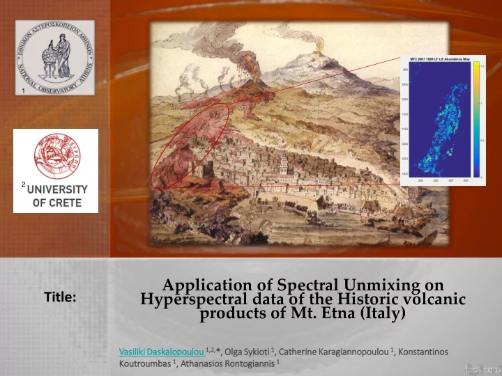
Application of Spectral Unmixing on Hyperspectral data of the Historic volcanic products of Mt. Etna (Italy)

Title:

Vas asiliki Das askal alopoulou 1,2,*, , Ol Olga Syki ykioti 1, Cath theri rine Kar aragi giannopoulou 1, Konstan antinos Koutr troumbas as 1, Athanasi asios s Rontogi giannis 1

1 2

A. Geological Setting B. Problem Definition

C. Data

D. Methodology E. Results

F. Discussion

2

Outline

Research Goals

• Delineate volcanic products with the use of Unmixing
• Accurate estimation of Abundances of deposited volcanic products
• Test different Signal Transformations to achieve optimum unmixing

results

• Determine the degree of correlation between LFs
• Qualitative overview of the volcanic surface complexity
• Extract underlying information of sub-pixel analysis, wrt to ground

truth

• Paradigm shift → future extension to younger, more correlated,

Lavas

3

4

• A. GEOLOGICAL SETTING

• Mt. Etna(1)

5

Subduction of the Ionian lithospheric slab beneath the Aeolian slab

• Mt. Etna(2)

6

Tectonic edifice of the Central Mediterranean Sea, the location

• f Mt. Etna is highlighted with red (from Branca et al, 2011 ).

• 4 major craters →

Northeast Crater (NEC), Voragine, Bocca Nuova and the Southeast Crater (SEC)

• Produce: voluminous Summit eruptions,

Paroxysmal events, Lava flows, Lava fountains

• Most eruptive: SEC
• > 300 secondary flank craters
• Flank

eruptions: historically more hazardous for populated regions

7 (modified by Spinetti et al., 2009)

• Mt. Etna(3)

Volcano’s Plumbing System

8 (modified by Ferlito et al., 2013)

Subduction forces the deep magmatic material to resurface. Central conduit system is located west of the most active volcanic region, Valle del Bove (VdB) and is:  7 Km x 5 Km wide and 1000 m deep Consists of: Intracrustal reservoirs and levels of exsolution for various gases.

Volcanic Activity

 Volcanism started  500 ka ago  Etna’s historical record of eruptive activity is well documented, with many attempts to identify systematic trends.  The post 1600 AD eruptive period is subdivided into 4 cycles.

9

First Period: 1600 – 1669 AD Second Period: 1669 – 1763 AD Third Period: 1755 – 1865 AD Fourth Period: 1865 – Present

Volcanic activity Summit Craters Degassing phases Strombolian Activity Lava Fountains Lava Overflows Flank eruptions Paroxysmal Eruptive events Lava flows

10

 Volcanic products : I. Lava Flows (LFs) occur from both summit and flank activity, subject to weathering, alteration and vegetation cover ⇒ morphology II. Pyroclastics are violent movement of gaseous compounds enriched with volcanic material, deposited on top of lava fields. III. Surface ash and scoriae !

Volcanic Products

Emerging lava: ‘a’a type → basaltic, rough surface, broken lava blocks & sharp texture

< 10% pahoehoe type → ropy, smoother

• surface. Flows

downwards → cools and may change to ‘a’a

11 (from Sgavetti et al., 2006 )

Spectral Signatures of Volcanic Products

Major Volcanic Formations

 1:50.000 scale Geological Map of Etna (Branca et. al, 2011) → Ground Truth

• 5 geological stages: Pre – Etnian activity, Fusion of four major

stratovolcanoes: Trifoglietto I, Trifoglietto II, Calanna and Mongibello Recent edifice bulk comprised of 2 volcanoes:

• Ellitico Volcano: distinguishable, steep slopes, mainly summit portion,

flanks reach the Alcantara river on the north.

• Mongibello Volcano: formed during the last 15 ka, covers  85% of

previous landforms, VdB dominates the Eastern side. 122 BC eruption revealed the Torre del Filosofo formation.

12

13

Major Volcanic Formations(2)

14

Torre del Filosofo MF1

Volcanic Products between

122 BC-1669 AD MF2 1669 AD-1971 AD MF3 1971 AD- Present

 Selected Formation MF1, 1536-1669 AD

MF1 Historic Lava Flows (1)

 Flank eruptions spanning 1536-1669 AD.

• 1536 AD

Overflown summit at NW, NE and flank eruption at  2200-1500 m. Extensive damage.

• 1537 AD

S flank vents at  1900-1700 m, destroyed Nicolosi, total length of 15 Km, largely buried under 1892 lava.

• 1566 AD

NE flank eruption, multiple fissures. Largely covered.

15

MF1 Historic Lava Flows (2)

 Flank eruptions spanning 1536, 1537 & 1566 AD (from left to right)

16

17

• 1610 AD

SW flank vent at 2350-1950m, 2 fissures. Destroyed cultivated vineyards Total lava vol. = 120 𝑦 106𝑛3

• 1614-24 AD

NW-W flanks at 2500-2000m, voluminous. Mostly pahoehoe. No damages reported.

• 1634-36 AD

S-SSE flank, short fissure at 2090-1975m, damage across. Total lava vol. = 150 𝑦 106𝑛3

• 1646-47 AD

NNE flank at 1900m, several villages destroyed. Prominent pyroclastic cone. Total lava vol. = 190 𝑦 106𝑛3

MF1 Historic Lava Flows(3)

18

MF1 Historic Lava Flows(4)

Flank eruptions 1610, 1614-24, 1634-36 & 1646-47 AD

19 (Fresco from Catania Cathedral)

MF1 Historic Lava Flows(3)

• 1669 AD:

Vigorous seismicity, S summit  800m. Destroyed Nicolosi, broke into Catania walls. Most devastating/voluminous, extensive lava field. Total lava vol. = 607 𝑦 106𝑛3

20

• B. PROBLEM DEFINITION

21

HSI CUBE

IDENTIFY LAVA FIELDS MIXED PIXELS FIND PURE COMPONENTS SPECTRAL UNMIXING ABUNDANCES ESTIMATION

SIGNAL TRANSFORMATIONS

Spectral Mixture Models

Spectral Mixing: each image pixel may contain one or more LC components ∴ mixed spectral characteristics

• Several Mixture Models depending
• n the mixed pixel morphology
• Solution: soft sub-pixel classification

techniques partition each pixel on different classes (UNMIXING)

22

Mixture Models Linear Bilinear

Linear Mixture Model (LMM)

 Assumption: each endmember covers a defined region within the pixel area & multiple scattering is negligible → Pure components Linearly mixed  Representation per pixel: 𝐳 = 𝐍𝒃 + 𝐨

• N: # of bands
• r=1,…K: # of endmembers,

 Potentially induced Constraint:

23

𝑏 ≥ 0 𝑂𝑂𝐷 , for every image pixel

N x 1 pixel signature vector N x K matrix: contains K 𝑛𝑠 = [𝑛1,𝑠, … , 𝑛𝑂,𝑠]𝑈 endmember signatures [𝑏1, . . , 𝑏𝐿]𝑈fractional abundance vector additive white noise

24

Bilinear Mixture Model (BMM)

 Assumption: linear components as in LMM + endmember correlation terms

 Formula:

𝐳 = 𝐍𝒃 +

i=1 K−1 j=i+1 K

𝑏𝑗,𝑘𝐧𝐣 ⊙ 𝐧𝐤 + 𝐨 ⇔ 𝐳 =

k=1 𝐿∗

𝑏𝑙∗𝐧𝐥∗ + 𝐨

where 𝐧𝐣 ⊙ 𝐧𝐤 denotes the ith & jth endmember interaction.  Potentially induced Constraint:

𝐿∗ = 1 2 𝐿(𝐿 + 1)

𝑏𝑙∗ ≥ 0

25

• C. DATA

Data

 Used: Hyperspectral image cube over Eastern Sicily, 09/07/2007  Big Data manipulation  From: NASA EO-1 HYPERION sensor

– 220 calibrated spectral bands (out of 242) – 10 nm spectral res. from 0.4 to 2.5 microns – 30 m spatial res. over a 7.7 Km swath – Highest SNR on Vis-VNIR – Level 1T radiometric & geometrically corrected product

Total # of bands : 140 after bad or noisy band

exclusion

26

The followed preprocessing steps:

• Atmospheric Correction (via FLAASH algorithm): Radiance

Reflectance1

• Water vapor and Cloud Masking
• Dimensionality / Noise Reduction via PCA: first 4 PCs Inverse PCA
• Vegetation Masking via NDVI: vegetated areas threshold on 0.41
• Active Areas Segregation: VdB omitted as a separate ROI
• Formation Masking: MF1 manually digitized, masked initial image

27

Data Preprocessing

1 not prerequisite step for unmixing analysis

28

a) from K. Karagiannopoulou, (2017). "Use of Hyperion spectral signatures and Sentinel-1 Polarimetric backscatter for lava flow differentiation in Mt. Etna, Sicily“.

a. b. c.

29

• D. METHODOLOGY

30

 Criteria of ROI selection:

• Dense Lava deposits, close to geological

map dates

• Avoid Borderline regions
• ROI > 30 pxls, otherwise merging
• Spectral profile inspection → minimum

variability

• Include populated environments

 # of ROIs = 13, for 9 LFs, 2 scoria cones and industrial, semi-urban, tile rooftops.

Endmember Extraction(1)

Endmember Extraction(2)

31

 Endmembers:

• Pixel values of the same ROI follow a Normal Distribution
• Assumed the majority of spectral information is between ±25% from

the mean value → resize each ROI  HOW ?

• Find the Gaussian borders → exclude the outliers
• Calculate new ROI average
• Mean value represents the 1x140 Endmember vector
• Not physical image pixel

 More efficient than simple averaging or median value

Volcanic Products Spectra

32

• Flat | slightly convex profile in 750-2500nm range
• Potential olivine presence: absorption feature on  900nm, need continuum removal
• Higher overall refl.: Tile rooftop buildings, Lowest overall refl.: 1610 scoria cone
• Older LFs have higher reflectance (consistent)

Volcanic Products Spectra

33

•  vegetation absorption: all products except industrial areas and 1536, 1669 LFs
• Alteration on: 1536, 1537, 1566, 1610, 1634-36, 1646-47 LFs
• Band reduction excludes crucial bands for compositional analysis

Linear Least Squares Unmixing (LLSU)

 Solution to mixed pixels problem: Linear Least Squares Unmixing

– Quadratic optimization problem + linear inequality constraints – Seeks the Optimum Abundance vector

 Minimize Least Squares Error (LSE): 𝑀𝑇𝐹 = 𝐍𝑏 − 𝐳 T 𝐍𝑏 − 𝐳 , 𝑡𝑣𝑐𝑘𝑓𝑑𝑢 𝑢𝑝 𝑏 ≥ 0

Constrained abundance vector estimation:

𝑏𝑂𝐷𝑀𝑇 = 𝐍T𝐍

−1𝐍T𝐳 − 𝐍T𝐍 −1

 Non-negativity constrained LS on Matlab via lsqnonneg2

35

2 STOC not included

Signal Transformations (1)

 Methods used on LLSU: 1. Raw Data - Channel Domain Representation

 Simple and robust

2. Reduced Channel Domain

 Exploit the HSI spectral redundancy  Dimensionality reduction via Feature Selection (FS)* → 22 optimum bands  Majority of information in R-VNIR !

3. FFT transformed Image Spectra

 DFT from Channel Domain → Frequency Domain  LLSU Frequency Domain ∝ LLSU Channel Domain

36 * Special Thanks to Dr. Kostas Themelis and Dr. Irida Xenaki for providing their scripts.

Signal Transformations(2)

 Methods used on LLSU: 4. FFT on Visible-VNIR

 Subspace identification ⇒ selection of bands with low SNR → for the Hyperion dataset VIS-VNIR  High-pass filter that enhances spectral details

5. FFT on Reduced Frequency Domain

 No significant variation over the 20th → Dimensionality Reduction

6. IFFT transformed Image

 Keep Bands with significant energy content  Reduced Frequency Domain → Initial Channel Domain

37

Signal Transformations(3)

 Methods used on Bilinear LSU: 7. Reduced Channel Domain

 Dot product of each endmember with the rest as 𝑛𝑗⨀𝑛𝑘 = Endmember Correlation  Non-Linearity is induced by the enhanced Endmember matrix

8. Augmented Spectral Signatures Domain

 Dot product of each of the bands = Band Correlation

38

39

Image Reconstruction

HOW ?

Endmember Matrix x Extracted Abundance Matrix– Neglect additional noise

• Unmixing Quality Assessment → Structural Similarity Index (SSIM)
• Quantitative measure of the comparison between the Initial image and

each Reconstructed image.

• Calculated on various windows of an image
• Formula based on three terms: luminance (𝒎), contrast (𝒅) & structure (𝒕)

HERE:

 Plot SSIM values for each of the 140 bands + mean SSIM values display.

40

• E. RESULTS

41

• METH. 1 Abundance Maps(1)
• LF colorbars are integrated on the same maximum value, unique for each method
• Generally: LFs are delineated
• Refined detail not provided by Geological Map
• High abundances on ROI areas, as expected

• METH. 1 Abundance Maps(2)

42

• METH. 3 Abundance Maps(1)

43

• Lava flows outline is maintained, lower abundances on same pixels
• Lava patterns are consistent
• Outline fades, 1634-36 LF → Gaussian noise reduction, stripping exists

• METH. 3 Abundance Maps(2)

44

• METH. 7 Abundance Maps(1)

45

• Homogeneous LF distribution
• Delineated lavas
• Sharper features on volcanic surface due to high frequency spectra
• Comparable abundances with previous methods

• METH. 7 Abundance Maps(2)

46

Faint 1610 scoria, low reflectance → spectrally correlated with other products

47

Comparative Analysis (1)

Comparative Analysis (2)

48

• Spatially uncorrelated lavas on

Geo, seem to be correlated !

• Underlying information?
• Break the homogeneity of the

Geo map

All Methods Image Reconstruction

49

• Reconstruction levels > 99.5% → successful unmixing processes
• Ascending trend until 1350nm, generally descending on low frequencies
• IFFT lowest SSIM due to zero pudding, 20 → 140 bands
• Reduced FFT (20 freq.) gives the same results as FFT

50

All Methods Image Reconstruction

• Bilinear Unmixing on the enhanced domain → Best overall reconstruction accuracy
• Note: Bilinear SSIM > LS SSIM → bilinear model as a better representation

 Meth. 2, 7 & 8 → subspace, give equivalent results

Time efficiency and Noise Reduction

51

Elapsed Time (sec) MEAN STDV LS 15.094 ± 0.235 LS Reduced 12.497 ± 0.161 FFT 14.168 ± 0.034 V_VNIR FFT 14.199 ± 0.123 20freq 12.342 ± 0.149 IFFT 15.325 ± 0.314 BL 32.919 ± 0.343 BL_aug 15.949 ± 0.177

 TIME EFFICIENT DIMENSIONALITY REDUCTION  TIME EFFICIENCT  TIME EFFICIENT & NOISE REDUCTION

52

• F. CONCLUSIONS &

DISCUSSION

Conclusions

 To sum up:

• Mapping of the different volcanic products wrt to Geological map
• Extract abundances of LF components, determine their spatial distribution
• Qualitative overview of the volcanic surface complexity
• Added value on existing context, quantitative information
• Achieve time efficient and robust techniques with comparable unmixing results
• Perform Dimensionality Reduction with very low computational cost → Big

Data efficient manipulation

• Created a Paradigm shift → Future extension

53

Discussion

 To the best of our knowledge:

 Volcanic products of Etna are studied mostly from field measurements, complimented by satellite images, in terms of mineralogical composition.  There are no references of Hyperspectral Unmixing techniques on Etnian Lava Fields, potentially to no other volcanic edifice.  Innovative work in terms of signal processing approaches tailored on a multidiverse volcanic environment.

54

Future Work

To compliment the HSI content:

 Sentinel-2 data provide great potential on the field  Constant coverage and high spatial resolution → Lava Discrimination  Performed already similar techniques on Multispectral data  Preliminary work on Etna with S2 data, that ultimately aims on:

55

Thank you for your attention !

Appendix

57

Key Points

• RESEARCH GOALS
• STUDY AREA “1536” to “1669” HISTORIC VOLCANIC PRODUCTS
• PROBLEM DEFINITION
• DATA PREPROCESSING
• MAIN DATA PROCESSING
• SPECTRAL MIXTURE MODELS: LINEAR & BILINEAR
• BHB
• RESULTS ABUNDANCE MAPS/METHOD
• COMPARATIVE ANALYSIS
• CONCLUSIONS
• DISCUSSION
• FUTURE WORK

METHODS

SIGNAL TRANSFORMATIONS LEAST SQUARES SPECTRAL UNMIXING IMAGE RECONSTRUCTION

58

(from Branca et al, 2011 ). 59

Etna’s Supersynthems

 LLSU on the:

1. Untransformed Channel Domain of the initial image 2. Reduced Channel Domain

 Exploit the HSI spectral redundancy  Perform Dimensionality reduction via Feature Selection (FS)*  Feature Selection uses the sparsity induced Fast Bi-ICE algorithm*, implemented in NOA  Output: vectors most significant Bands & Ranks  Optimum Band number: 22 Bands  1st FS band (41) = 973 nm (0.1918), 22nd FS band (31) = 783 nm (0.1648)

 Channel Domain reduced to corresponding 22 bands.  Majority of information in R-VNIR !

60

Signal Transformations(2)

* Special Thanks to Dr. Kostas Themelis and Dr. Irida Xenaki for providing their scripts.

 LLSU on the:

1. Untransformed Channel Domain of the initial image 2. Reduced Channel Domain

 Exploit the HSI spectral redundancy  Perform Dimensionality reduction via Feature Selection (FS)*  Feature Selection uses the sparsity induced Fast Bi-ICE algorithm*, implemented in NOA  Output: vectors most significant Bands & Ranks  Optimum Band number: 22 Bands  1st FS band (41) = 973 nm (0.1918), 22nd FS band (31) = 783 nm (0.1648)

 Channel Domain reduced to corresponding 22 bands.  Majority of information in R-VNIR !

61

Signal Transformations(3)

* Special Thanks to Dr. Kostas Themelis and Dr. Irida Xenaki for providing their scripts.

 TIME EFFICIENCY

 LLSU on the:

3. FFT transformed entire Image

 DFT from Channel Domain → Frequency Domain  Reduce complexity to 𝑷(𝒐𝒎𝒑𝒉𝒐)  Perform FFT on the endmember matrix too  LLSU on the abs amplitude values of the Image - Endmember vectors  LLSU Frequency Domain ∝ LLSU Untransformed  Does it give quantitatively the same results?

4. FFT on the Visible-VNIR part of the spectrum

 # of endmembers is related to the dimension of the subspace occupied by measurements  Subspace identification ⇒ selection of bands with low SNR → for the Hyperion dataset VIS-VNIR

62

Signal Transformations(4)

 LLSU on the:

3. FFT transformed entire Image

 DFT from Channel Domain → Frequency Domain  Reduce complexity to 𝑷(𝒐𝒎𝒑𝒉𝒐)  Perform FFT on the endmember matrix too  LLSU on the abs amplitude values of the Image - Endmember vectors  LLSU Frequency Domain ∝ LLSU Untransformed  Does it give quantitatively the same results?

4. FFT on the Visible-VNIR part of the spectrum

 # of endmembers is related to the dimension of the subspace occupied by measurements  Subspace identification ⇒ selection of bands with low SNR → for the Hyperion dataset VIS-VNIR (a priori known)

63

Signal Transformations(5)

64

 LLSU on the:

 76 first bands  Essentially a High-pass filter that enhances spectral details  FFT on reduced bands computationally low-cost  Reducing Gaussian Image noise  Stripping effect remains (High Frequency noise)

5. Reduced Frequency Domain via FFT

 Plot the FFT frequencies of the Endmember Matrix  20 First → signal’s major energy content  No significant variation over the 20th → Dimensionality Reduction  Comparable results with the FFT on entire image

Signal Transformations(6)

 TIME EFFICIENT NOISE REDUCTION

65

 LLSU on the:

 76 first bands  Essentially a High-pass filter that enhances spectral details  FFT on reduced bands computationally low-cost  Reducing Gaussian Image noise  Stripping effect remains (High Frequency noise)

5. Reduced Frequency Domain via FFT

 Plot the FFT frequencies of the Endmember Matrix  20 First → signal’s major energy content  No significant variation over the 20th → Dimensionality Reduction  Comparable results with the FFT on entire image

Signal Transformations(7)

66

Signal Transformations(8)

 LLSU on the:

6. IFFT transformed Image

 From the diminished 20 freq. domain → 140 Channel domain  Return to the initial image through zero padding the FFT transformed image  Keep only the energy dominant bands

 Bilinear LSU on the:

7. Reduced Channel Domain

 Exploit the FS reduced domain  Compute the Enhanced Endmember Matrix  Dot product of each endmember with the rest as Xi.*Xj = Endmember Correlation  Non-Linearity is induced by the enhanced Endmember matrix  Flexible model for multi-correlated LFs  TIME EFFICIENT DIMENSIONALITY REDUCTION

67

Signal Transformations(9)

 LLSU on the:

6. IFFT transformed Image

 From the diminished 20 freq. domain → 140 Channel domain  Return to the initial image through zero padding the FFT transformed image  Keep only the energy dominant bands

 Bilinear LSU on the:

7. Reduced Channel Domain

 Exploit the FS reduced domain  Compute the Enhanced Endmember Matrix  Dot product of each endmember with the rest as Xi.*Xj = Endmember Correlation

68

Signal Transformations(10)

 Non-Linearity is induced by the enhanced Endmember matrix  Flexible model for multi-correlated LFs

 Bilinear LSU on the:

8. Augmented Spectral Signatures Domain

 Endmember matrix and Image spectral enhancement  Again compute the dot product of each of the bands = Band Correlation  Non-Linearity is induced by the augmented Endmember matrix

LLSU Untransformed Abundance Maps

69

70

LLSU Untransformed Abundance Maps

71

LLSU Untransformed Abundance Maps

72

LLSU Untransformed Abundance Maps

73

LLSU Untransformed Abundance Maps