
SLIDE 1
Automatic Control EEM 3117
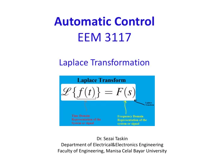
Laplace Transformation
- Dr. Sezai Taskin
Department of Electrical&Electronics Engineering Faculty of Engineering, Manisa Celal Bayar University
EEM 3117 Laplace Transformation Dr. Sezai Taskin Department of - - PowerPoint PPT Presentation
Automatic Control EEM 3117 Laplace Transformation Dr. Sezai Taskin Department of Electrical&Electronics Engineering Faculty of Engineering, Manisa Celal Bayar University Laplace Transformation The Laplace transform of a function f ( t ),
Department of Electrical&Electronics Engineering Faculty of Engineering, Manisa Celal Bayar University
Slides 2 2
[ ( )] ( ) ( )
st
f t F s f t e dt
L
Slides 2 3
Slides 2 4
1 ( ) ( ) t f t u t t
[1] 1 1
st st
e dt e s s s s
L
Slides 2 5
( ) ( )
( ) [ ] ( ) 1 ( ) ( ) 1
at at at st s a t s a t
f t e e e e dt e dt e s a s a s a s a
L
at
Slides 2 6
at
at
Slides 2 7
2 2
2 2
Slides 2 8
st st t
Slides 2 9
( ) ( ) t t f t u t t
(integration by parts)
2
[ ] 1
st st st st
t e t dt e t e e t d dt s s s s
L
1
n n
similarly
Slides 2 10
1 2 ( 1)
n n n n n n
Slides 2 11
t
as
Slides 2 12
Laplace Transformation Algebraic Manipulation Inverse Laplace Particular Integral Complementary function
Slides 2 13
2 2 2
t t t t t
Transformed Solution Transformed Equation
Slides 2 14
1 2 1 2
( ) ( ). ( ) ( ) ( ) ( ) F s F s F s f t f t f t Ex:
2 2 1 2 2( ) 2 2 2
1 1 1 ( ) 3 2 ( 1) ( 2) ( ) ( ) ( ) ( 1)
t t t t t t t t t t t
F s s s s s f t e e f f t d e e d e e d e e e e