[PDF] - EE 6882 Visual Search Engine Prof. Shih Fu Chang, Feb. 6 th 2012 PDF Document

SLIDE 1

2/6/2012 1

EE 6882 Visual Search Engine

Prof. Shih‐Fu Chang, Feb. 6th 2012

Lecture #3

 Evaluation Metrics  Local Features: Corner Detector, SIFT  Local Feature Matching

(Many slides from A. Efors, W. Freeman, C. Kambhamettu, L. Xie, and likely others) (Slides preparation assisted by Rong‐Rong Ji)

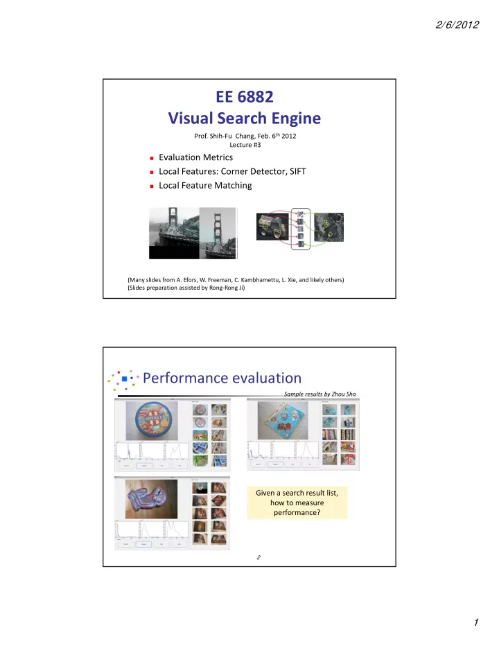
Performance evaluation

2

Given a search result list, how to measure performance?

Sample results by Zhou Sha

SLIDE 2

2/6/2012 2

Evaluation



Detection



False Alarms



Misses



Correct Dismissals

2 / ) ( ) /( ) /( ) /(

1

R P R P F B A B F B A A P C A A R         

1

N

" Irrelevant " Relevant" " 1    n Vn

B V D A V C V B V A

N n n N n n K n n K n n

       

   

       

) ) 1 ( ( ) ( ) 1 (

1 1 1 1

N Images K Results



Recall



Precision



False



Combined D

B

C

A

“Returned” “Relevant Results” Ground truth search DB

Evaluation Measures

Precision at depth K Precision Recall Curve Receiver Operating Characteristic (ROC Curve)

P

R

K V P

k n n k

/ ) (

1

 

  R (Recall) F (false)

SLIDE 3

2/6/2012 3

Average Precision

Ranked list of results

3/7 3/6 3/5 3/4 2/3 1/2 1/1 Precision 1 1 1 truth Ground D D D D D

s

... ...

21 63 8 15

data relevant

f

# : ) ( ) , min( 1

1

total R V P R K AP

j K j j





 

AP approximates areas under PR curve

1 2 3 4 5 6 7 Precision j

3  

i

P AP

1.0

Example:

Evaluation Metric: Average Precision

 Observations (AP)

 AP depends on the rankings of relevant data and the size of the

relevant data set. E.g., R= 10

Case I:

+ + + + + + + + + +

Case II:

+ - + - + - + - + - + - + - + - + - +

Case III:

- -
+

+ + + + + + + +

- -
Case IV:
- -
+

+ + + + +

…

Case V:

- -
+

+ + + + +

…

+ + + Affected by ranks Same top ranks, different recall

SLIDE 4

2/6/2012 4

Texture



What is texture?



“stylized subelements, repeated in meaningful ways”



May have quasi‐stochastic macro structure (e.g. bricks), each with stochastic micro structure



Why texture?



Application to satellite images, medical images



Useful for describing and reproducing contents of real world images, i.e., clouds, fabrics, surfaces, wood, stone



Challenging issues



Rotation and scale variance (3D)



Segmentation/extraction of texture regions from images



Texture in noise

A wide range of filters for textures



Tamura Texture



Zernike moments



Steerable filters



Ring/wedge filters



Gabor filter banks



wavelet transforms

Randen, T. and Husøy, J. H. 1999. Filtering for Texture Classification: A Comparative Study. IEEE Trans. Pattern Anal. Mach. Intell. 21, 4 (Apr. 1999), 291‐310.



Quadrature mirror filters



Discrete cosine transform



Co-occurrence matrices

SLIDE 5

2/6/2012 5

Filter approaches for texture description



Fourier Transform F(u,v) Energy Distribution

 Angular features (directionality)  Radial features (coarseness) 2 1 1 2

tan , ) , (

2 1

 

        





u v where dudv v u F V

2 2 2 1 2

, ) , (

2 1

r v u r where dudv v u F V r

r

    

x



y





x



y



r

Gabor filters

 Gaussian windowed Fourier Transform

 Dyadic partitions of the spatio‐frequency space  Basis filters are product/conv of Fourier basis images and Gaussians

x

=

Different Frequency

Gabor filters

) 2 /( 1 ); 2 /( 1

y v x u

     

SLIDE 6

2/6/2012 6

Example: Filter Responses

from Forsyth & Ponce

Filter bank Input image

Local Features

 What are good local features?

 Distinct, interesting content  Repeatable (invariant)  Precise locations – sensitive to position shift

 Aperture Problem – information within a small window often

insufficient for determining true motion or matching

shift up shift left

Images of Elizabeth Johnson

The barber pole illusion

Multiple motion hypotheses exist Corners help

SLIDE 7

2/6/2012 7

Corner Detection

 Types of local image windows

 Flat: Little or no brightness change  Edge: Strong brightness change in single direction  Flow: Parallel stripes  Corner/spot: Strong brightness changes in orthogonal

directions

 Basic idea

 Find points where two edges meet  Look at the gradient behavior over a small window

(Slide of A. Efros)

Harris Detector: Basic Idea

“flat” region: no change in all directions “edge”: no change along the edge direction “corner”: significant change in all directions

(Slide of A. Efros)

SLIDE 8

2/6/2012 8

Harris Detector: Mathematics

 

2 ,

( , ) ( , ) ( , ) ( , )

x y

E u v w x y I x u y v I x y    



Change of intensity for the shift [u,v]:

Intensity Shifted intensity Window function

r

Window function w(x,y) = Gaussian 1 in window, 0 outside

Harris Corner Detector

 Taylor’s expansion 2 , 2 2 2 ,

( , ) ( , )[ ( , ) ( , )] ( , )[ ( , )]

x y x y x y

E u v w x y I x u y v I x y w x y I u I v O u v       

 

2 , 2 , ,

2 2 ( , ) 2 ( , ) ( , ) ( , ) ( , ) ( , ) ( , ) ( , )

x x y y x y x y x y

E u v Au Cuv Bv A w x y I x y B w x y I x y C w x y I x y I x y      

  

SLIDE 9

2/6/2012 9

Harris Detector: Mathematics

 

( , ) , u E u v u v M v       

Taylor’s Expansion: For small shifts [u,v] we have a bilinear approximation: 2 2 ,

( , )

x x y x y x y y

I I I M w x y I I I         



where M is a 22 matrix computed from image derivatives:

Harris Detector: Mathematics

 

( , ) , u E u v u v M v       

Intensity change in shifting window: eigenvalue analysis 1 > 2 – eigenvalues of M

(1)-1/2 (2)-1/2

Ellipse E(u,v) = const

If we try every possible shift, the direction of fastest change is 1

(Slide of K. Efros)

SLIDE 10

2/6/2012 10

Harris Detector: Mathematics

1 2 “Corner” 1 and 2 are large, 1 ~ 2; E increases in all

directions

1 and 2 are small; E is almost constant

in all directions

“Edge” 1 >> 2 “Edge” 2 >> 1 “Flat” region Classification of image points using eigenvalues of M:

(Slide of A. Efros) 

Model image sequence as a spatiotemporal function I(x,y,t)

 Assume no change at displaced point, similar optical flow in local area

where

Harris Detector: Another Interpretation- Optical Flow

Opt ical Flow

dI I dx I dy I dt x dt y dt t          dI dt 

x y t

I u I v I   

( , ) ( , ) dx dy u v dt dt 

SLIDE 11

2/6/2012 11

 Lucas-Kanade Tracking: local consistency of optical flow

Harris Detector: Interpretation based on Tracking

– (u,v) remain constant within a local patch 

 Optimal (u, v) satisfies Lucas-Kanade equation

2 ( , ) ( , ) ,

E(u,v)= ( )

x y t u v u v x y

Min Min I u I v I



 



x x x y x t x x y y y t

I I I I I I u I I I I I I v                    

     

(Slide of W. Freeman)

M

Conditions for solvability

 Optimal (u, v) satisfies Lucas-Kanade equation  When is this Solvable?



M should be invertible



eigenvalues 1, 2 of M should not be too small



M should be well-conditioned



1/2 should not be too large (1 = larger eigenvalue)

(Slide of Khurram Hassan-Shafique)

SLIDE 12

2/6/2012 12

Harris Detector: Mathematics

Measure of corner response:

 

2

det trace R M k M   det Trace M R M 

(k – empirical constant, k = 0.04-0.06) 1 2 1 2

det trace M M       

Or 1 2 1 2

det trace M M       

Harris Detector: Mathematics

1 2 “Corner” “Edge” “Edge” “Flat”

R depends only on eigenvalues of

M

R is large for a corner
R is negative with large

magnitude for an edge

|R| is small for a flat region

R > 0 R < 0 R < 0 |R| small

(Slide of K. Efros)

SLIDE 13

2/6/2012 13

Edge

– large gradients, all the same

– large 1, small 2

Low texture region

– gradients have small magnitude

– small 1, small 2

SLIDE 14

2/6/2012 14

High textured region

– gradients are different, large magnitudes

– large 1, large 2

Harris Detector: Summary



Average intensity change in direction [u,v] can be expressed as a bilinear form:



Describe a point in terms of eigenvalues of M: measure of corner response



A good (corner) point should have a large intensity change in all directions, i.e. R should be large positive

 

( , ) , u E u v u v M v       

 

2 1 2 1 2

R k       

(Slide of K. Efros) 2 2 ,

( , )

x x y x y x y y

I I I M w x y I I I         



(k – empirical constant, k = 0.04-0.06)

SLIDE 15

2/6/2012 15

Harris Detector

 The Algorithm:

 Find points with large corner response function R

(R > threshold)

 Take the points of local maxima of R

Models of Image Change

 Geometry

 Rotation  Similarity (rotation + uniform scale)  Affine (scale dependent on direction)

valid for: orthographic camera, locally planar

bject

 Photometry

 Affine intensity change (I  a I + b)

(Slide of C. Kambhamettu)

SLIDE 16

2/6/2012 16

Harris Detector: Some Properties

 Rotation invariance

Ellipse rotates but its shape (i.e. eigenvalues) remains the same Corner response R is invariant to image rotation

(Slide of C. Kambhamettu)

Harris Detector: Some Properties

 Partial invariance to affine intensity change

 Only derivatives are used => invariance to intensity shift I  I + b  Intensity scale: I  a I R x (image coordinate)

threshold

R x (image coordinate)

(Slide of C. Kambhamettu)

SLIDE 17

2/6/2012 17

Harris Detector: Some Properties

 But: non-invariant to image scale!

All points will be classified as edges

Corner !

(Slide of C. Kambhamettu)

Scale Invariant Detection



Consider regions (e.g. circles) of different sizes around a point



Regions of corresponding sizes (at different scales) will look the same in both images

Fine/Low Coarse/High

(Slide of C. Kambhamettu)

SLIDE 18

2/6/2012 18

Scale Invariant Detection



The problem: how do we choose corresponding circles

independently in each image?

(Slide of C. Kambhamettu)

Reading List

Rui, Y., T.S. Huang, and S.‐F. Chang, Image retrieval: current techniques, promising

directions and open issues. Journal of Visual Communication and Image Representation, 1999. 10(4): p. 39‐62.

Smith, J.R. and S.‐F. Chang. VisualSEEk: a Fully Automated Content‐Based Image

Query System. in ACM International Conference on Multimedia. 1996. Boston, MA.

David G. Lowe, Distinctive Image Features from Scale‐Invariant Keypoints,

International Journal of Computer Vision, 60(2), 2004, pp91‐110.

Randen, T. and J. Husoy, Filtering for texture classification: A comparative study.

Pattern Analysis and Machine Intelligence, IEEE Transactions on, 2002. 21(4): p. 291‐310.

Mikolajczyk, K. and C. Schmid, A performance evaluation of local descriptors. IEEE

Transactions on Pattern Analysis and Machine Intelligence, 2005: p. 1615‐1630.

Brown, M., R. Szeliski, and S. Winder. Multi‐image matching using multi‐scale
riented patches. in IEEE CVPR. 2005.
Interesting demo:

Georg Klein and David Murray, “Parallel Tracking and Mapping for Small AR Workspaces,” ISMAR 2007.