EE 6882 Visual Search Engine Prof. Shih Fu Chang, Feb. 13 th 2012 - - PDF document

SLIDE 1

2/13/2012 1

EE 6882 Visual Search Engine

• Prof. Shih‐Fu Chang, Feb. 13th 2012

Lecture #4

 Local Feature Matching  Bag of Word image representation: coding and pooling

(Many slides from A. Efors, W. Freeman, C. Kambhamettu, L. Xie, and likely others) (Slides preparation assisted by Rong‐Rong Ji)

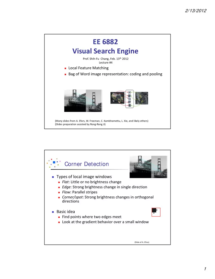
Corner Detection

 Types of local image windows

 Flat: Little or no brightness change  Edge: Strong brightness change in single direction  Flow: Parallel stripes  Corner/spot: Strong brightness changes in orthogonal

directions

 Basic idea

 Find points where two edges meet  Look at the gradient behavior over a small window

(Slide of A. Efros)

SLIDE 2

2/13/2012 2

Harris Detector: Mathematics

 

2 ,

( , ) ( , ) ( , ) ( , )

x y

E u v w x y I x u y v I x y    



Change of intensity for the shift [u,v]:

Intensity Shifted intensity Window function

• r

Window function w(x,y) = Gaussian 1 in window, 0 outside

Harris Detector: Mathematics

 

( , ) , u E u v u v M v       

Taylor’s Expansion: For small shifts [u,v] we have a bilinear approximation: 2 2 ,

( , )

x x y x y x y y

I I I M w x y I I I         



where M is a 22 matrix computed from image derivatives:

SLIDE 3

2/13/2012 3

Harris Detector: Mathematics

 

( , ) , u E u v u v M v       

Intensity change in shifting window: eigenvalue analysis 1 > 2 – eigenvalues of M

(1)-1/2 (2)-1/2

Ellipse E(u,v) = const

If we try every possible shift, the direction of fastest change is 1

(Slide of K. Efros)

Harris Detector: Mathematics

Measure of corner response:

 

2

det trace R M k M   det Trace M R M 

(k – empirical constant, k = 0.04-0.06) 1 2 1 2

det trace M M       

Or 1 2 1 2

det trace M M       

SLIDE 4

2/13/2012 4

Harris Detector

 The Algorithm:

 Find points with large corner response function R

(R > threshold)

 Take the points of local maxima of R

Models of Image Change

 Geometry

 Rotation  Similarity (rotation + uniform scale)  Affine (scale dependent on direction)

valid for: orthographic camera, locally planar

• bject

 Photometry

 Affine intensity change (I  a I + b)

(Slide of C. Kambhamettu)

SLIDE 5

2/13/2012 5

Harris Detector: Some Properties

 But: non-invariant to image scale!

All points will be classified as edges

Corner !

(Slide of C. Kambhamettu)

Scale Invariant Detection



Consider regions (e.g. circles) of different sizes around a point



Regions of corresponding sizes (at different scales) will look the same in both images

Fine/Low Coarse/High

(Slide of C. Kambhamettu)

SLIDE 6

2/13/2012 6

Scale Invariant Detection



The problem: how do we choose corresponding circles

independently in each image?

(Slide of C. Kambhamettu)

Scale-Space Pyrimad

SLIDE 7

2/13/2012 7

Scale Space: Difference of Guassian

2 2 2

1 2 2

( , , )

x y

G x y e

 



 





Functions for determining scale

2 2 2

1 2 2

( , , )

x y

G x y e

 



 



 

2

( , , ) ( , , )

xx yy

L G x y G x y      ( , , ) ( , , ) DoG G x y k G x y    

Kernel Image f  

Kernels:

where Gaussian Note: both kernels are invariant to scale and rotation (Laplacian) (Difference of Gaussians)

Scale Invariant Detection

(Slide of C. Kambhamettu)

SLIDE 8

2/13/2012 8

Gausian Kernel, DOG

Sigma 2 Sigma 4 Diff Sigma2-Sigma4

Difference of Gaussian, DOG

SLIDE 9

2/13/2012 9



Detect maxima and minima of difference-of-Gaussian in scale space

B l u r R e s a m p l e S u b t r a c t

Key Point Localization Scale Invariant Interest Point Detectors



Harris-Laplacian1

Find local maximum of:



Harris corner detector in space (image coordinates)



Laplacian in scale

1 K.Mikolajczyk, C.Schmid. “Indexing Based on Scale Invariant Interest Points”. ICCV 2001 2 D.Lowe. “Distinctive Image Features from Scale-Invariant Keypoints”. IJCV 2004

scale

x y

 Harris   Laplacian 

• SIFT (Lowe)2

Find local maximum of: – Difference of Gaussians in space and scale scale

x y

 DoG   DoG 

(Slide of C. Kambhamettu)

SLIDE 10

2/13/2012 10

Scale Invariant Detectors

K.Mikolajczyk, C.Schmid. “Indexing Based on Scale Invariant Interest Points”. ICCV 2001



Experimental evaluation of detectors w.r.t. scale change

Repeatability rate:

# correct correspondences avg # detected points

SIFT keypoints

SLIDE 11

2/13/2012 11

After extrema detection After curvature, edge responses

SLIDE 12

2/13/2012 12

Keypoints orientation and scale SIFT Invariant Descriptors

Dominant direction

• f gradient
• Extract image patches relative to local
• rientation

SLIDE 13

2/13/2012 13

Local Appearance Descriptor (SIFT)

[Lowe, ICCV 1999]

Histogram of oriented gradients over local grids

• e.g., 4x4 grids and 8 directions

‐> 4x4x8=128 dimensions

• Scale invariant

S.-F. Chang, Columbia U. 25

Compute gradient in a local patch

Point Descriptors



We know how to detect points



Next question:

How to match them?

?



Point descriptor should be:



Invariant



Distinctive

SLIDE 14

2/13/2012 14

Feature matching

?

Slide of A. Efros

Feature-space outlier rejection [Lowe, 1999]:

• 1-NN: SSD of the closest match
• 2-NN: SSD of the second-closest match
• Look at how much the best match (1-NN) is than the 2nd best

match (2-NN), e.g. 1-NN/2-NN

Slide of A. Efros

SLIDE 15

2/13/2012 15

Feature-space outliner rejection

Can we now compute H from the blue points?

• No! Still too many outliers…
• What can we do?

Slide of A. Efros

RANSAC for estimating homography

RANSAC loop: 1. Select four feature pairs (at random) 2. Compute homography H (exact) 3. Compute inliers where SSD(pi’, H pi) < ε 4. Keep largest set of inliers 5. Re-compute least-squares H estimate on all of the inliers

Slide of A. Efros

SLIDE 16

2/13/2012 16

Least squares fit

Find “average” translation vector

Slide of A. Efros

RANSAC

Slide of A. Efros

SLIDE 17

2/13/2012 17

From local features to Visual Words

…

clustering 128‐D feature space visual word vocabulary

K-Mean Clustering

 Training data  Unsupervised learning  K‐mean clustering

 Fix K value  Initialize the representative of each cluster  Map samples to closest cluster  Re‐compute the centers



Can be used to initialize other clustering methods

   

( )

i

x label i ? 

x(1) x(2)

• +

+ + ++

• +

+ + + +

…

• C1

C2 C3 CK 1 2

, ,..., , , ) , ), '

N i k i k i k'

x x x samples for i=1,2,...,N, x C if Dist(x C Dist(x C k k end   

SLIDE 18

2/13/2012 18

Sivic and Zisserman, “Video Google”, 2006

Visual Words: Image Patch Patterns

Corners Blobs eyes letters

Represent Image as Bag of Words

…

clustering keypoint features visual words

… …

BoW histogram

SLIDE 19

2/13/2012 19

Pooling Binary Features

Consider PxK matrix P: # of features, K: # of codewords To begin with simple model, assume vi are iid.

Boureau, Jean Ponce, Yann LeCun, A Theoretical Analysis of Feature Pooling in Visual Recognition, ICML 2010

• …
• …
• …

Distribution Separability

Better separability achieved by

• 1. increasing the distance between the means of the two class‐

conditional distributions

• 2. reducing their standard deviations.

SLIDE 20

2/13/2012 20

Average pooling: Max pooling:

Distribution Separability

Class separability

SLIDE 21

2/13/2012 21 For binary features: For continuous features:

• Modeling will be more complex and the conclusions are slightly

different

Soft Coding

Image source: http://www.cs.joensuu.fi/pages/franti/vq/lkm15.gif

• - Assign a feature to multiple visual

words

• - weights are determined by

feature-to-word similarity

Details in: Jiang, Ngo and Yang, ACM CIVR 2007.

42

SLIDE 22

2/13/2012 22

Multi‐BoW Spatial Pyramid Kernel

• a

43

• S. Lazebnik, et al, CVPR 2006

Classifiers

• K‐Nearest Neighbors + Voting
• Linear Discriminative Model (SVM)

44

SLIDE 23

2/13/2012 23

to maximize margin

wTx + b = 0

Airplane

Machine Learning: Build Classifier

wTxi + b > 0 if label yi= +1 wTxi + b < 0 if label yi= ‐1 Find separating hyperplane: w Decision function: f(x) = sign(wTx + b)

Support Vector Machine (tutorial by Burges ‘98)

:

t

Decision boundary H b + = w x



Look for separation plane with the highest margin



Linearly separable

1

hyperplane ( ) : 1

t i

H H b

+

+ = + w x



Two parallel hyperplanes defining the margin

2

hyperplane ( ) : 1

t i

H H b

• +

= - w x



Margin: sum of distances of the closest points to the separation plane

margin = 2/ w



Best plane defined by w and b

wTxi + b > 1 if label yi= +1 wTxi + b < ‐1 if label yi= ‐1 yi (wTxi + b) > 1 for all xi

SLIDE 24

2/13/2012 24    

if 0, is on

• r

and is a support vector

i i

H H a

+

• >

x



Weight sum from positive class = Weight sum from negative class



Direction of w: roughly from negative support vectors to positive ones

Max Margin Solution for separable case



How to compute w and b?



How to classify new data? w

∗

Non-separable

Lagrange multiplier: minimize

if 1, then is misclassified (i.e. training error)

i i

x  

Ensure positivity



Add slack variables

i

x

New objective function

SLIDE 25

2/13/2012 25

 All the points located in the margin gap or

the wrong side will get

i

C  

What if C increases?

i

C  

i

C   



When C increases, samples with errors get more weights

 better training accuracy, but smaller margin  less generalization performance

after C increases

Generalized Linear Discriminant Functions

1

( ) ( )

d t i i i

g a y

=

= =

å

x x a y

)



I nclude more than just the linear terms

1 1 1

( )

d d d t t i i ij i j i i j

g w w x w x x w

= = =

= + + = + +

å å å

x w x x Wx



I n general



Example



Shape of decision boundary

 ellipsoid, hyperhyperboloid, lines etc

[ ]

2 1 2 3 2 1 2 3

( ) 1

t

g x a a x a x a a a x x = + + é ù = ê ú ë û

[ ] [ ]

1 1 2 2 3 1 2 1 2 3 1 1 2

( ) 1

t

g x a x a x a x x a a a x x x = + + =



Data become separable in higher-dimensional space

 learning parameters in high dimension is hard

(curse of dim.)

 instead, try to maximize margins  SVM

Figure from Duda, Hart, and Stork

SLIDE 26

2/13/2012 26

Non-Linear Space

Map to a high dimensional space, to make the data separable

1 1 1 1 1 1

1 ( ) ( ) 2 1 ( , ) 2

l l l D i i j i j i j i i j l l l i i j i j i j i i j

L y y y y K a a a a a a

= = = = = =

=

• F

×F =

• å

å å å å å

x x x x



Find the SVM in the high-dim space (embedding space)



Luckily, we don’t have to find

1

( ) nor ( )

l i i i i i

y a

=

F F

å

s s



We can use the same method to maximize LD to find

i

a

1

( ) ( ) ( )

s

N i i i i

g y b a

=

= F ×F +

å

x s x



I nstead, we define kernel

( , ) ( ) ( )

i i

K = F × F s x s x

1

( ) ( , )

s

N i i i i

g y K b a

=

Þ = +

å

x s x

w

Some popular kernels

Cubic polynomial separable non-separable

polynomial Gaussian Radial Basis Function (RBF) sigmoidal neural network

SLIDE 27

2/13/2012 27

i

C  

i

C   



SVM Classifier is completely determined by the training samples that are on the hyperplanes or within the margin

* 1 l i i i i

y a

=

= å w x

yi (w Txi + b) < = 1

Reading List

• Lazebnik, S., C. Schmid, and J. Ponce. Beyond bags of features: Spatial pyramid matching for

recognizing natural scene categories. in IEEE CVPR. 2006.

• Jiang, Y., C. Ngo, and J. Yang. Towards optimal bag‐of‐features for object categorization and

semantic video retrieval. in ACM CIVR. 2007.

• Chang, S., et al. Columbia University/VIREO‐CityU/IRIT TRECVID2008 high‐level feature

extraction and interactive video search. in NIST TRECVID Workshop. 2008.

• Jiang, Y., et al. Columbia‐UCF TRECVID2010 Multimedia Event Detection: Combining Multiple

Modalities, Contextual Concepts, and Temporal Matching. in TRECVID Workshop. 2010.

• Pattern Classification, 2nd ed., Richard O. Duda, Peter E. Hart, and David G. Stork ISBN: 0‐

471‐05669‐3, 2000, Wiley

• Viola, P. and M. Jones. Rapid Object Detection using a Boosted Cascade of Simple Features. in

Proceedings IEEE Conf. on Computer Vision and Pattern Recognition. 2001.

• Yan, R., J. Yang, and A.G. Hauptmann. Learning Query‐Class Dependent Weights in Automatic

Video Retrieval. in ACM Multimedia. 2004. New York.