EE 6882 Visual Search Engine Prof. Shih Fu Chang, Jan. 30, 2012 - PDF document

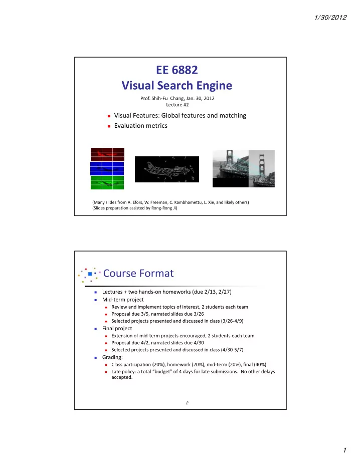
1/30/2012 EE 6882 Visual Search Engine Prof. Shih ‐ Fu Chang, Jan. 30, 2012 Lecture #2  Visual Features: Global features and matching  Evaluation metrics (Many slides from A. Efors, W. Freeman, C. Kambhamettu, L. Xie, and likely others) (Slides preparation assisted by Rong ‐ Rong Ji) Course Format Lectures + two hands ‐ on homeworks (due 2/13, 2/27)  Mid ‐ term project  Review and implement topics of interest, 2 students each team  Proposal due 3/5, narrated slides due 3/26  Selected projects presented and discussed in class (3/26 ‐ 4/9)  Final project  Extension of mid ‐ term projects encouraged, 2 students each team  Proposal due 4/2, narrated slides due 4/30  Selected projects presented and discussed in class (4/30 ‐ 5/7)  Grading:  Class participation (20%), homework (20%), mid ‐ term (20%), final (40%)  Late policy: a total “budget” of 4 days for late submissions. No other delays  accepted. 2 1

1/30/2012 1 0.8 0.6 0.4 0.2 Image Features 0 0 20 40 60 80 100  Why features are needed?  Finding similar images in database  Classifying images to categories merl.com  Tracking objects in video  Creating panorama  Stereo matching ‐ > 3D  Desired properties photoguides.net  Compact (~100 – 1000 dimensions)  Easy to compute (30 fps for video)  Robust (invariant to photometric, geometric, content variations) 3 Desired Properties of Visual Features Invariance:   Rotation, scaling, cropping, shift, etc.  illumination, pose, clutter, occlusion, viewpoint 2

1/30/2012 Invariant Local Features Image content is transformed into local feature coordinates that are invariant to translation, rotation, scale, and other imaging parameters Features Descriptors (Slide of A. Efros) (review) Imaging Formation DSP R G R G R G B G B G (White Image irradiance R G R G R Balance, G B G B G intensity Contrast R G R G R Camera CCD Additive Demosaicking Enhancement Lens Response Sensor Noise … etc) Filter Function 6 3

1/30/2012 Color Spaces and Color Order Systems  Color Spaces  RGB – cube in Euclidean space R G B    r g b       R G B R G B R G B  Standard representation used in color displays  Drawbacks  RGB basis not related to human color judgments  Intensity should be one of the dimensions of color  Important perceptual components of color are hue, saturation, and brightness  Perceptual color spaces: HIS, HSV Understanding HSI from RGB Turn the RGB cube so that Black ‐  White axis is vertical Each plane containing the B ‐ W axis  and a color point contains all the colors of the same hue Hue represented as angle between  the plane and a reference plane (e.g. Red) Saturation: distance to axis, less  saturated by mixing more grey colors Intensity measured by intersection  with the B ‐ W axis. Cross section shape:  triangle – hexagon ‐ triangle Images from Gonzalez and Woods 8 4

1/30/2012 Colors on the HSI color cone Cross section approximated by triangle or  circle HSI values computed by various  geometrical models, e.g.,       I 1 / 3 1 / 3 1 / 3 R V   1 2 H tan ( )          V 1 / 6 1 / 6 2 / 6 G V       1 1         2  2 1 / 2  V   1 / 6 1 / 6 0   B  Chroma ( V V ) 2 1 2 More suitable for measuring perceptual  distance Can be quantized unevenly, e.g.,  Columbia VisualSEEK System: 16M colors (in RGB) quantized to 166 HSV colors (18 Hue, 3 Sat, 3 Val, 4 Gray) 9 Manipulations in the HSI space Hue of Green & Blue set to 0.  Saturation of Cyan reduced by  HSI values of  half. primary/secondary colors Intensity of White reduced by  HSI allows independent  half. manipulations of colors 10 5

1/30/2012 Color Histogram Feature extraction from color images   Choose GOOD color space  Quantize color space to reduce number of colors      1 if I [ , ] m n r I , [ , ] m n g I , [ , ] m n b  R G B  [ , , ] h r g b RGB  0 otherwise m n Invariance?   Scale, shift, rotation, crop, view angle, illumination, clutter, occlusion Advantages   Easy to compute and compare Cons   Lack spatial information, dimension may be high Color Moments  Is there a more compact representation than color histogram?  Compute moment statistics in each color channel. ? 6

1/30/2012 Localizing http://www.ai.mit.edu/courses/6.801/Fall2002/ Color Layout Search Columbia VisualSEEk (Smith & Chang, ’96) IBM QBIC (Flickner et al ’95) Query results 7

1/30/2012 Color correlogram http://www.ai.mit.edu/courses/6.801/Fall2002/ http://www.ai.mit.edu/courses/6.801/Fall2002/ 8

1/30/2012 http://www.ai.mit.edu/courses/6.801/Fall2002/ Color Coherence Vector (CCV) (Pass et a l, 1997) B C B B A A Not just 2 1 2 2 1 1 B B C B A A count of 2 2 1 2 1 1 colors, also Region segmentation B C D B A A 2 1 3 2 1 1 check B B B A A E 2 2 2 1 1 3 adjacency 2 2 1 1 3 3 B B A A E E 2 2 1 1 3 3 B B A A E E regions A B C D E color 1 2 3 Coherent! 1 2 1 3 3 color  12 15 5 CCV Size threshold: 3 12 15 3 1 5 size  3 0 1                        G , ,..., , G , ,..., , 1 1 1 1 I n n I n n n n                           ฀ ฀ = = G i i i i H i i i i   i 1 i 1    by triangular inequality G H 9

1/30/2012 Distance Metrics between 1 0.8 0.6 Feature Vectors 0.4 0.2 0 0 20 40 60 80 100    p 1 / p ( ( ) ( ) ) D x i x i L p distance  1 2 p i Quadratic distance       ( ( ) ( ) ( , ) ( ) ( ) ) D x i x i C i j x j x j 1 2 1 2 q j i        T C(i,j): color distance ( ) ( ) x x C x x 1 2 1 2 Histogram Intersection  Mohalanobis distance  where C x is the covariance matrix Normalize distance in the major/minor axes Mohalanobis Metric      T 2   1  D x x C x x mah 1 2 x 1 2   (1,1) (1,2) ... (1, ) c c c d   d: dimension of features   covariance matrix C ... ... ... ...  x    ( ,1) ( ,2) ... ( , )  c d c d c d d N          c i j ( , )  x ( ) i m i ( )   x ( ) j m j ( )  N / 1, N number of samples : k k  1 k x j x j x j x j x j o o o o o o o o oo oo o o o o o o o o o o o o o x i x i x i x i x i 1 c    1  0 c s s    c s s c s s c s s i j i j i j i j 2 2 s i , s j : std. deviation 10

1/30/2012 Mohalanobis Metric where C x is the covariance matrix       T         | ...| ( , ,..., ) | ...| C  e e e  diag  e e e  x 1 2 d 1 2 d 1 2 d         T 1       1   | ...| ( ( , ,..., )) | ...| C  e e e  diag  e e e  x 1 2 d 1 2 d 1 2 d e 2 e 1 Normalize distance in the eigen vector axes Project data to the eigen vectors, divide with the sd of each eigen dimension, and compute Euclidian distance Mohalanobis Metric (cont.) . cm . Advantages of Mahalanobis metric . .  . . . . . . .. .  Account for scaling of coordinate axes . .. .. .  Invariant under linear transformation km    2  2 T , If y Ax C AC A D D . . . ... y x y x . .  Correct for correlation . . . . . .. . . ..  Produce curved as well as linear decision boundaries m 1 Maha. Dist. x i c 1 Selected class Minimum m c Selector Maha. Dist.  c c Potential issue   Need enough training data to estimate Cov. Matrix 11