Economics 2 Professor Christina Romer Spring 2019 Professor David - PDF document
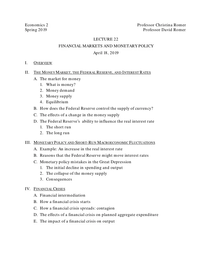
Economics 2 Professor Christina Romer Spring 2019 Professor David Romer LECTURE 22 FINANCIAL MARKETS AND MONETARY POLICY April 18, 2019 I. O VERVIEW II. T HE M ONEY M ARKET , THE F EDERAL R ESERVE , AND I NTEREST R ATES A. The market for
Economics 2 Professor Christina Romer Spring 2019 Professor David Romer LECTURE 22 FINANCIAL MARKETS AND MONETARY POLICY April 18, 2019 I. O VERVIEW II. T HE M ONEY M ARKET , THE F EDERAL R ESERVE , AND I NTEREST R ATES A. The market for money 1. What is money? 2. Money demand 3. Money supply 4. Equilibrium B. How does the Federal Reserve control the supply of currency? C. The effects of a change in the money supply D. The Federal Reserve’s ability to influence the real interest rate 1. The short run 2. The long run III. M ONETARY P OLICY AND S HORT -R UN M ACROECONOMIC F LUCTUATIONS A. Example: An increase in the real interest rate B. Reasons that the Federal Reserve might move interest rates C. Monetary policy mistakes in the Great Depression 1. The initial decline in spending and output 2. The collapse of the money supply 3. Consequences IV. F INANCIAL C RISES A. Financial intermediation B. How a financial crisis starts C. How a financial crisis spreads: contagion D. The effects of a financial crisis on planned aggregate expenditure E. The impact of a financial crisis on output
Economics 2 Christina Romer Spring 2019 David Romer L ECTURE 22 Financial Markets and Monetary Policy April 18, 2019
Announcement • Problem Set 5 is due now.
I. O VERVIEW
Determination of Short-Run Output: The “Keynesian Cross” PAE Y=PAE PAE Y 1 Y
Two More Things that Can Shift PAE • Monetary Policy: Actions taken by the central bank to affect nominal and real interest rates. • Disruptions in Financial Markets: Specifically, a financial crisis.
Two Key Ideas Concerning Monetary Policy in the Short Run • By changing the money supply, the central bank can change the real interest rate. • A change in the real interest rate shifts the PAE curve in the Keynesian cross diagram, and so changes output in the short run.
II. T HE M ONEY M ARKET , THE F EDERAL R ESERVE , AND I NTEREST R ATES
Economists’ Definition of “Money” • Assets that can be used to make purchases. • Concretely, you can usually think of money as meaning currency.
The Nominal Interest Rate and Money Demand • Because you don’t earn interest on cash, the opportunity cost of holding money is what you could earn on other assets. • That is, the opportunity cost of holding money is the nominal interest rate. • So: Money demand is a decreasing function of the nominal interest rate.
The Demand for Money i MD M
Money Supply • At any point in time, the amount of currency available is just a number. • Determined by the central bank. • That is, we take the quantity of money supplied as given.
The Supply of Money i MS M
Equilibrium in the Market for Money i MS i 1 MD M 1 M
How Does the Federal Reserve Change the Money Supply? • Open market operation: The buying and selling of government bonds by the central bank. • When the Federal Reserve sells bonds, the money supply decreases. • When the Federal Reserve buys bonds, the money supply increases.
A Decrease in the Money Supply i MS 2 MS 1 i 2 i 1 MD M 2 M 1 M The Fed sells bonds.
The Fed’s Ability to Influence the Real Interest Rate—the Short Run • By changing the money supply, the Fed can change the nominal interest rate, i. • Recall: r = i − π (or r = i − π e ), and there is nominal rigidity (inflation only changes slowly). • So: When the Fed changes i, it changes r.
In the Short Run, Nominal and Real Interest Rates Generally Move Together Nominal Real Source: FRED.
The Fed’s Ability to Influence the Real Interest Rate—the Short Run versus the Long Run • As we have just seen, the Fed can affect the real interest rate in the short run. • However, in the long run, r must be at the level that equilibrates S* and I*. • The Fed cannot keep r away from this level indefinitely. • We will discuss next week what prevents the Fed from doing this.
III. M ONETARY P OLICY AND S HORT - RUN M ACROECONOMIC F LUCTUATIONS
The Real Interest Rate and Planned Aggregate Expenditure (PAE) Recall: PAE = C + I p + G + NX. • I p is lower when r is higher. • Saving is higher when r is higher, so C is lower when r is higher. • We will see two weeks from now that NX is lower when r is higher. Conclusion: An increase in r reduces PAE at a given Y.
An Increase in the Real Interest Rate PAE Y=PAE PAE 1 PAE 2 Y 2 Y* Y
Monetary Policy • Actions taken by the central bank to affect nominal and real interest rates. • Contractionary monetary policy: Federal Reserve actions to increase nominal and real interest rates. • Expansionary monetary policy: Federal Reserve actions to decrease nominal and real interest rates.
Why Might the Central Bank Undertake Expansionary or Contractionary Monetary Policy? • To offset some other force that is shifting the PAE line (countercyclical monetary policy). • We’ll disucss an example next time (monetary policy in the Great Recession). • To pursue some other objective. • We’ll discuss this extensively next week (the Fed’s concern with inflation). • A mistake. • Example: Monetary policy in the Great Depression.
Industrial Production, 1927–1934 9.0 8.0 Index (2012=100) 7.0 6.0 5.0 4.0 3.0 1927 1928 1929 1930 1931 1932 1933 1934 Source: Federal Reserve Bank of St. Louis, FRED.
The Money Stock, 1923–1933 50 48 46 44 Billions of Dollars 42 40 38 36 34 32 30 1923 1924 1925 1926 1927 1928 1929 1930 1931 1932 1933 Source: Federal Reserve Bank of St. Louis, FRED.
Real Interest Rate, 1923–1933 16 14 12 10 Percent 8 6 4 2 0 -2 1923 1924 1925 1926 1927 1928 1929 1930 1931 1932 1933 Source: Federal Reserve Bank of St. Louis, FRED.
Monetary Contraction in the Great Depression PAE Y=PAE PAE 1 PAE 2 Y 2 Y* Y PAE 2 shows the effects of the fall in autonomous consumption.
Monetary Contraction in the Great Depression PAE Y=PAE PAE 1 PAE 2 PAE 3 Y 3 Y 2 Y* Y PAE 3 shows the effect of monetary contraction and the rise in r.
Industrial Production, 1927–1934 9.0 8.0 Index (2012=100) 7.0 6.0 5.0 4.0 3.0 1927 1928 1929 1930 1931 1932 1933 1934 Source: Federal Reserve Bank of St. Louis, FRED.
IV. F INANCIAL C RISES
Financial Intermediation • The process of getting saving into productive investment. • Financial intermediaries are the markets and institutions that do this. • Financial intermediaries include banks, investment banks, money market mutual funds, pension funds, etc.
What Is a Financial Crisis? • A time when: • A number of financial institutions are in danger of failing. • People lose confidence in many financial institutions. • As a result, there is widespread disruption of financial intermediation.
How Individual Financial Institutions Can Fail • Defaults and changes in asset values can reduce the value of an institution’s loans and securities. • If the value of the loans and securities falls to the point where they are worth less than the institution’s obligations to its depositors and lenders, the institution is insolvent. • A belief that the institution is in danger of becoming insolvent can cause depositors to withdraw their funds and lenders to stop lending—which can cause the insolvency to occur.
Source: Federal Reserve Bank of St. Louis, FRED. Case-Shiller House Price Index, January 2000 = 100 100 150 200 250 50 0 Jan-87 House Prices, 1987–2015 Jan-89 Jan-91 Jan-93 Jan-95 Jan-97 Jan-99 Jan-01 April 2006 Jan-03 Jan-05 Jan-07 Jan-09 Jan-11 Jan-13 Jan-15
Source: http://www.housingviews.com.
Contagion of Crises across Financial Institutions • Confidence: Troubles at one institution create doubts about the health of other institutions, even if there are no connections between them. • Linkage: Troubles at one institution directly harm other institutions because of loans, insurance contracts, and other direct links among them. • Fire Sale: Troubles at one institution cause it to sell off assets, driving down the prices of assets held by other institutions. • Macroeconomic: Troubles at one institution reduce PAE and hence Y, and so harm other institutions.
Deposits in Failed or Suspended Banks, 1927-1933 500 450 400 350 Millions of Dollars 300 250 200 150 100 50 0 1927 1928 1929 1930 1931 1932 1933 Source: Federal Reserve.
Effects of a Financial Crisis on PAE • It raises credit spreads. • It may raise lending standards or otherwise reduce the availability of loans. • It may harm consumer and firm confidence. • All of these developments are likely to reduce PAE at a given level of Y.
Credit Spreads during the 2008 Financial Crisis Source: Economic Report of the President , February 2010.
Tightening Loan Standards during the 2008 Financial Crisis Source: Federal Reserve, Senior Loan Officer Opinion Survey, January 2018.
Decline in the Number of Banks in the Great Depression Number of Banks (1000s) Source: www.econreview.com.
Recommend
More recommend
Explore More Topics
Stay informed with curated content and fresh updates.
