economics 2 professor christina romer spring 2017
play

Economics 2 Professor Christina Romer Spring 2017 Professor David - PDF document

Economics 2 Professor Christina Romer Spring 2017 Professor David Romer LECTURE 15 MACROECONOMIC VARIABLES AND ISSUES March 9, 2017 I. M ACROECONOMICS VERSUS M ICROECONOMICS II. R EAL GDP A. Definition B. Nominal GDP and real GDP C. A little


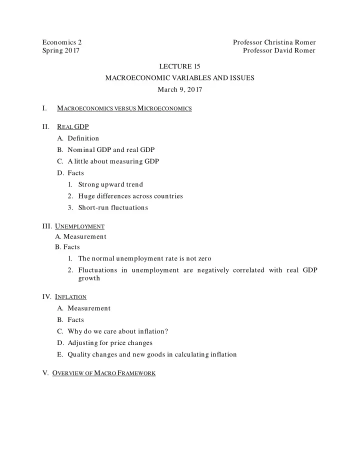
  1. Economics 2 Professor Christina Romer Spring 2017 Professor David Romer LECTURE 15 MACROECONOMIC VARIABLES AND ISSUES March 9, 2017 I. M ACROECONOMICS VERSUS M ICROECONOMICS II. R EAL GDP A. Definition B. Nominal GDP and real GDP C. A little about measuring GDP D. Facts 1. Strong upward trend 2. Huge differences across countries 3. Short-run fluctuations III. U NEMPLOYMENT A. Measurement B. Facts 1. The normal unemployment rate is not zero 2. Fluctuations in unemployment are negatively correlated with real GDP growth IV. I NFLATION A. Measurement B. Facts C. Why do we care about inflation? D. Adjusting for price changes E. Quality changes and new goods in calculating inflation V. O VERVIEW OF M ACRO F RAMEWORK

  2. Economics 2 Christina Romer Spring 2017 David Romer L ECTURE 15 Macroeconomic Variables and Issues March 9, 2017

  3. Announcements • Research reading for Tuesday, March 14 (by William Nordhaus): • Read only the assigned pages. • Read for approach and findings; think about relevance for the measurement of inflation and growth in standards of living.

  4. I. M ACROECONOMICS VERSUS M ICROECONOMICS

  5. Macroeconomics • Definition: • The study of the aggregate economy. • Concerned with: • Total output. • Aggregate price level and inflation. • The unemployment rate. • The overall level of interest rates; the exchange rate; overall exports and imports.

  6. II. R EAL GDP

  7. Real Gross Domestic Product (Real GDP) • The market value of the final goods and services newly produced in a country during some period of time, adjusted for price changes.

  8. Nominal GDP • Nominal GDP: The market value of the final goods and services newly produced in a country during some period of time, not adjusted for price changes. • Thus, for the United States, it is measured in dollars. • Example: Nominal GDP in 2016 = ∑ P i , 2016 • Q i , 2016 , i where i represents each possible good in the economy (and ∑ is the symbol for a sum). • Note that we use 2016 prices in computing 2016 nominal GDP, 2015 prices in computing 2015 nominal GDP, ….

  9. Calculating Real GDP • Choose a base year (for example, 2009), and always use prices from the base year to multiply the quantities. • Example: If 2009 is the base year: 2016 real GDP = ∑ P i , 2009 • Q i , 2016 . i • That is, if 2009 is the base year, 2016 real GDP is the answer to the question, “How much would all the final goods and services newly produced in the United States in 2016 have been worth at 2009 prices?”

  10. Growth Rate of Real GDP • The percentage change in real GDP from one year to the next.

  11. A Little about Measuring GDP • Key points: • Final goods and services. • Newly produced . • Within the country . • In some period of time .

  12. 3 Approaches to Measuring GDP • Expenditure: Use market prices and the quantities of final goods. • Can divide into consumption (C), investment (I), government purchases (G), and net exports (NX). • Production (value added): follow goods through each stage of production. • Income: Income from producing new goods and services within the country. • Can divide into labor income and capital income.

  13. Real GDP in the United States, 1950–2016 Source: FRED (Federal Reserve Economic Data); data from Bureau of Economic Analysis.

  14. Real GDP per Capita in the U.S., 1950–2016 Source: FRED; data from Bureau of Economic Analysis.

  15. GDP per Capita over Time and Regions Source: Bloom and Sachs, “Geography, Demography, and Economic Growth in Africa.”

  16. U.S. Real GDP, 2004–2011 Source: FRED; data from Bureau of Economic Analysis.

  17. U.S. Real GDP, 1929–1940 Source: FRED; data from Bureau of Economic Analysis.

  18. U.S. Real GDP, 2011–2016 Source: FRED; data from Bureau of Economic Analysis.

  19. III. U NEMPLOYMENT

  20. Definitions • Employed: The number of people who are working. • Unemployed: The number of people who are not working and who are actively looking for work. • Labor force: Employed + unemployed. • Unemployment rate: u = Unemployed Labor force • 100.

  21. The U.S. Unemployment Rate, 1948–2017 Source: FRED; data from Bureau of Labor Statistics.

  22. The Natural Rate of Unemployment • The economy’s normal or usual unemployment rate. • The natural rate of unemployment is more than zero.

  23. Real GDP Growth (Percent, Red) and Change in the Unemp. Rate (Percentage Points, Blue), 1961–2016 Source: FRED; data from Bureau of Economic Analysis and Bureau of Labor Statistics.

  24. IV. I NFLATION

  25. Calculating the Consumer Price Index • Choose a base year (for example, 1983), and find the basket of goods and services households purchased in 1983. • Then the CPI in 2016 is: CPI 2016 = Price of 1983 market basket in 2016 Price of 1983 market basket in 1983 • 100. • That is, if 1983 is the base year, the 2016 CPI is the answer to the question, “By what ratio would households’ spending have to be higher in 2016 than it was in 1983 for them to buy the same things they bought in 1983?”

  26. Calculating the Consumer Price Index— Algebra • Choose a base year (for example, 1983), and always use quantities from the base year to multiply the prices. • Then the CPI in 2016 is: CPI 2016 = ∑ P i , 2016 • Q i , 1983 i • 100. ∑ P i , 1983 • Q i , 1983 i

  27. Inflation • The percent change in a price index. • Example: the inflation rate from 2015 to 2016 is: π 2016 = P 2016 − P 2015 • 100. P 2015 • Note: If inflation is negative, we say there is “deflation.”

  28. U.S. Inflation (Percent Change in the Price Index for Personal Consumption Expenditures), 1953–2016 Source: FRED; data from Bureau of Economic Analysis.

  29. U.S. Inflation (Percent Change in the Price Index for Personal Consumption Expenditures), 1930–1933 Source: FRED; data from Bureau of Economic Analysis.

  30. Why Do We Care about Inflation? • An argument for not caring. • Redistribution. • Psychology. • Efficiency.

  31. Adjusting Variables for Price Changes • What would $X in Year A be equivalent to in terms of Year B dollars? $X P B , P A where P A and P B are the price index in year A and year B. • Example: What was Richard Nixon’s final salary equivalent to in today’s dollars? • His salary was $200,000; the CPI in August 1974 was 49.9; the CPI now is 244.2. Thus: $200,000 244.2 49.9 = $979,000.

  32. Quality Changes and New Goods in Calculating Inflation • If the quality of a good improves and its price rises, we try to take out the part of the price increase that is due to the quality improvement (and count only the remainder in calculating inflation). • If there are new goods, we try to account for the fact that they give households a new way of obtaining utility.

  33. Quality Changes, New Goods, and Real GDP • We can think of real GDP as nominal GDP divided by a price index: • If 2009 is the base year, define: ∑ P i , t • Q i , t i GDP Price Index t = . ( ∗ ) ∑ P i , 2009 • Q i , t i • Then our earlier definition of real GDP implies : Nominal GDP t Real GDP t = . GDP Price Index t • In practice, rather than using a simple price index like ( * ), we use a price index that tries to account for quality changes and new goods.

  34. V. O VERVIEW OF M ACRO F RAMEWORK

  35. Determinants of the Long-Run Trend • Potential Output: The amount of output (real GDP) that the economy can produce when using its resources at normal rates. • Key resources: • Labor • Capital • Technology

  36. Determinants of Short-Run Fluctuations • Aggregate demand: The total demand for final goods and services. • Key features of the short-run model: • In the short run, output depends on aggregate demand. • Developments in the private sector, monetary policy, and fiscal policy all affect aggregate demand. • The level of output relative to potential affects inflation, which in turn affects aggregate demand through monetary policy.

  37. International Macroeconomics • Interactions between aggregate economies. • Key issues: • Exchange rates • The trade deficit or surplus

  38. Real Broad Effective Exchange Rate for the U.S., 1994–2017 Source: FRED; data from Bank of International Settlements.

  39. Net Exports as a Share of GDP, 1975–2016 Source: FRED; data from Bureau of Economic Analysis.

  40. The Federal Funds Rate, 1954–2017 Source: FRED; data from Board of Governors of the Federal Reserve System.

Download Presentation
Download Policy: The content available on the website is offered to you 'AS IS' for your personal information and use only. It cannot be commercialized, licensed, or distributed on other websites without prior consent from the author. To download a presentation, simply click this link. If you encounter any difficulties during the download process, it's possible that the publisher has removed the file from their server.

Recommend


More recommend