Economics 2 Professor Christina Romer Spring 2017 Professor David - PDF document

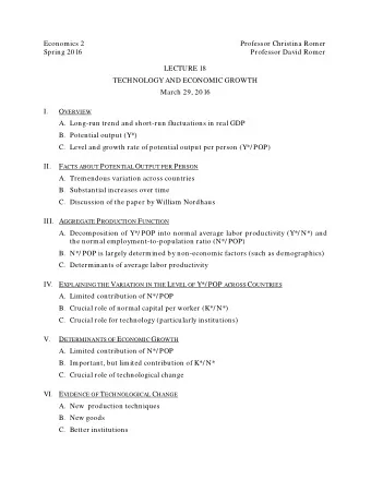
Economics 2 Professor Christina Romer Spring 2017 Professor David Romer LECTURE 13 LABOR AND WAGES March 2, 2017 I. O VERVIEW A. Another firm decision: How to produce the desired quantity B. The market for labor II. L ABOR D EMAND A. Marginal revenue product of labor B. Profit maximization C. Labor demand curve III. L ABOR S UPPLY A. Utility maximization B. Substitution and income effects of a wage increase C. Labor supply curve IV. L ABOR M ARKET E QUILIBRIUM V. E XAMPLES OF L ABOR M ARKET A NALYSIS A. Decline in demand for the product workers produce B. An increase in capital or technological progress C. A union negotiates a wage above the equilibrium level VI. T HE E FFECTS OF I NCREASED I MMIGRATION A. Theoretical impact of increased immigration B. Empirical evidence (Paper by David Card on the Mariel Boatlift)

Economics 2 Christina Romer Spring 2017 David Romer L ECTURE 13 Labor and Wages March 2, 2017

Announcements • Problem Set 3: • Due next Tuesday (March 7). • Problem set work session tomorrow (March 3), 4–6 p.m. in 648 Evans. • Journal article reading for next time: • Thomas Piketty and Emmanuel Saez, “Income Inequality in the United States, 1913–1998.”

I. O VERVIEW

Three Decisions of a Firm • How much to produce in the short run. • Whether to enter or exit in the long run. • How to produce the desired quantity. • How much of different inputs to use in the production process.

Market for Labor Wage S 1 (W) W 1 D 1 L 1 Employment (L)

We can talk about the labor market at different levels: • Market for labor in the whole economy. • Market for labor for a particular occupation or industry (plumbers, computer programmers, construction workers). • Market for workers with particular characteristics (teenagers, married women, low-skilled workers).

II. L ABOR D EMAND

Labor Demand Comes from Profit Maximization • What factors affect a firm’s demand for labor? • Demand for the product it produces • Productivity of labor • The wage and other labor costs • Profits are maximized where MR = MC. • Extension of this basic condition: Firms want to hire labor up to the point where the extra revenue generated by another worker is just equal to the extra cost.

Marginal Revenue Product of Labor (MRP L ) • The extra revenue generated by one more worker. • It is composed of two pieces: • Marginal product of labor (MP L ): The extra output produced by one more worker. • Marginal revenue (MR): The extra revenue from selling one more unit. • MRP L = MP L • MR

The Special Case of Perfect Competition: • For competitive firms: MR = P. • So for competitive firms: MRP L = MP L • P. • We call MP L • P the value of the marginal product of labor (VMP L ).

MRP L Declines as L Increases • MP L declines because of diminishing returns. • MR is either constant (for a competitive firm) or declining (for an imperfectly competitive firm). • So MRP L is declining.

MRP L for a Particular Firm MRP L MRP L l

Profit Maximization Implies: • Firms want to hire labor up to the point where: MRP L = W. • At each wage, a firm wants to hire whatever quantity of labor has a MRP L equal to that wage.

Labor Demand Curve for an Individual Firm W Firm’s Labor Demand Curve W 1 W 2 MRP L l 1 l 2 l

Labor Demand Curves Individual Firm Market W W MRP L ,D MRP L ,d l L

III. L ABOR S UPPLY

Labor supply behavior comes from utility maximization on the part of household • Think of a household choosing between leisure and everything else that it likes. • P Leisure is the wage. • Condition for utility maximization: MU Leisure MU Everything Else = P Leisure P Everything Else

MU Leisure MU Everything Else = P Leisure P Everything Else • Substitution Effect: When the wage rises, the consumer wants to substitute away from leisure (so work more). • Income Effect: When the wage rises, the consumer is richer and wants more leisure (so work less). • Which effect dominates is an empirical matter.

Labor Supply Curves Individual Household Market W W s S l L

IV. L ABOR M ARKET E QUILIBRIUM

Market for Construction Workers W S 1 W 1 D 1 L 1 L

V. E XAMPLES OF L ABOR M ARKET A NALYSIS

Example 1: Decrease in the Demand for the Product • Consider the market for construction workers. • The bursting of the housing bubble in 2008 led to a large decline in the demand for housing (and a fall in house prices). • What would you expect this to do to the employment and wages of construction workers?

Effect of a Decrease in Demand for the Product Market for Construction Output (Houses) P S 1 P 1 P 2 D 1 D 2 Q 2 Q 1 Q

Example 1: Decrease in the Demand for the Product (continued) • The fall in the price of the output lowers the MRP L at each level of employment. • The labor demand curve shifts back. • Wages and employment of construction workers both fall.

Effect of a Decrease in Demand for the Product Market for Construction Workers W S 1 W 1 W 1 D 1 D 2 L 2 L 1 L

Median Usual Weekly Earnings Construction Laborers Occupations 750 700 650 600 Dollars 550 500 450 400 2004 2005 2006 2007 2008 2009 2010 2011 2012 2013 2014 2015 2016 Source: FRED, Federal Reserve Bank of St. Louis

Example 2: Increase in Machines or Technological Progress • Consider the market for high-skilled workers. • Computer technology spread rapidly across many industries in the late 1980s and 1990s. • What would you expect this to do to the employment and wages of high-skilled workers whose jobs use computers (such as architects, engineers, and professors)?

Example 2: Increase in Machines or Technological Progress (continued) • The addition of machines or technological progress (or, often, both together) will increase the MP L . • In most circumstances, this will increase the MRP L . • This implies that the labor demand curve has shifted out. • Wages and employment of workers using the technology will rise.

Effect of an Increase in Capital (Computers) Market for High-Skilled Workers W S 1 W 2 W 1 D 2 D 1 L 1 L 2 L

Real Wages of Full-Time Male Workers by Educational Level Source: David Autor, “Skills, Education, and the Rise of Earnings Inequality among the “Other 99 Percent”

Example 2: Increase in Machines or Technological Progress (continued) • A possible complication involves the price of the output. • Increased labor productivity will shift out the supply curve for the product and reduce its price. • If the fall in the price is large, the increase in labor productivity could conceivably reduce MRP L . • This is not the normal outcome. Over history, technological progress has been good for workers’ wages.

Real Wages in the U.K. over the Very Long Run From: Clark, “The Condition of the Working Class in England, 1209-2004”

Example 3: A Union Negotiates a Wage about the Equilibrium Level • Consider the market for autoworkers. • Suppose that the autoworkers union negotiates a wage that is above the equilibrium level in this industry. • What would you expect this to do to the employment and wages of autoworkers?

Effect of a Negotiated Wage Market for Autoworkers W S 1 W N W 1 D 1 L D1 L 1 L S1 L

Example 3: A Union Negotiates a Wage about the Equilibrium Level (continued) • The negotiated wage is like a price floor. • It will raise the wage of workers who remain employed. • But, profit-maximizing firms won’t pay workers more than the MRP L of the last worker hired. Instead, they will cut back employment to L D1 . • We would expect increased unemployment among autoworkers.

VI. E FFECTS OF I NCREASED I MMIGRATION

Example 4: Increased Immigration Raises the Supply of Low-Skilled Workers • Suppose that immigration of low-skilled workers increases. • What would you expect this to do to the wages and employment of low-skilled workers?

Effect of Increased Immigration Market for Low-Skilled Workers W S 1 S 2 W 1 W 2 D 1 L 1 L 2 L

Empirical Evidence on the Impact of Immigration • Problems with previous studies: • Many looked at wages and immigration by city. • But, perhaps people chose to go to cities where labor demand was expanding. • Immigration could still be reducing wages of native workers relative to what they otherwise would have been.

Simultaneous Changes in Supply and Demand Market for Low-Skilled Workers W S 1 S 2 W 1 , W 2 D 2 D 1 L

Empirical Evidence on the Impact of Immigration • David Card paper uses a natural experiment: • Mariel Boatlift (May-September 1980). • 125,000 Cubans migrated to the U.S. • Almost all went to Miami. • No issue of immigrants choosing to go where the labor market was expanding. • Excellent data on wages and employment before and after the influx of immigrants.

Card Paper on the Effects of the Mariel Boatlift Source: David Card, “The Impact of the Mariel Boatlift on the Miami Labor Market”