DRAFT 19 October 2017 Please do not Cite. Results are preliminary. - - PDF document

SLIDE 1

DRAFT 19 October 2017 Please do not Cite. Results are preliminary. Background Paper to accompany poster at IUSSP Cape Town 2017 Fertility Responses to Child Deaths in Historical and Contemporary Populations George Alter, University of Michigan Estelle McLean, London School of Hygiene and Tropical Medicine and Malawi Epidemiology and Intervention Research Unit Aisha N.Z. Dasgupta, United Nations Population Division and London School of Hygiene and Tropical Medicine Descriptions of fertility transitions in Europe generally assume that birth control was used to avoid exceeding a desired family size. This implies that couples who suffered a child death would have been less likely to practice birth control than couples whose children survived. From this perspective the emergence of a “replacement effect” (i.e. higher fertility following a child death) is a sign of the practice of family limitation. Knodel (Knodel 1982; 1988) found much stronger evidence of a replacement effect among German village populations after fertility began to decline. Ethnographic research on Africa has encountered a very different response to child

• deaths. Bledsoe, Banja, and Hill (1998) describe a mother who began using modern

birth control following the death of her child in spite of a strong desire for more

• children. Concerned that repeated pregnancies were eroding her capacity for

childbearing, this woman believed that rest and recuperation were the best way to assure that her next pregnancy would be successful. The use of modern contraception for birth spacing has important implications for understanding the slow pace of fertility decline in Africa. As some observers predicted (Caldwell, Orubuloye and Caldwell 1992), fertility in African societies seems to be following a very different path than Europe and East Asia. This paper will look for the contrasting responses to child deaths described by Knodel and Bledsoe. Birth intervals have been reconstructed from a subset of Knodel’s German village genealogies which we contrast with data from the Karonga Health and Demographic Surveillance Site in northern Malawi. Our analysis employs the “split population” or “cure model,” a mover/stayer model in which covariates can have separate effects on “stopping” and “spacing” (Kuk and Chen 1992; Li and Choe 1997; Yamaguchi and Ferguson 1995). Since infant deaths tend to increase fertility by terminating breastfeeding, the estimation model uses time-varying covariates for child deaths and time since last birth. Two Models of Fertility and Birth Control We characterize Knodel’s (1982) description of the emergence of a child replacement effect as an extension of the “natural fertility hypothesis” proposed by Louis Henry (Henry 1961). Henry’s model emphasizes the shift to parity-dependent fertility control, which implies that couples begin aiming for a target family size. In this framework we

SLIDE 2

DRAFT 19 October 2017 Please do not Cite. Results are preliminary. expect a child replacement effect to emerge with the transition to family limitation. If fertility behavior is not being affected by family size, we do not expect behavior to change after the death of a child. We also examine other implications of the Natural Fertility Hypothesis, such as the prediction that fertility transitions occur because of ‘stopping’ rather than ‘spacing’ (Knodel and van de Walle 1979). Caroline Bledsoe and her co-authors have offered a very different description of fertility decisions of African women. Bledsoe, Banja, and Hill (1998) describe a mother who began using modern birth control following the death of her child in spite of a strong desire for more children. Concerned that repeated pregnancies were eroding her capacity for childbearing, this woman believed that rest and recuperation were the best way to assure that her next pregnancy would be successful (Bledsoe et al. 1998; Bledsoe and Banja 2002). Thus, modern contraception can be used with the intention of increasing rather than limiting family size. Bledoe’s (2002) account emphasizes the belief that a woman’s physical capacity for childbearing is limited and that adverse events, such as miscarriages and infant deaths, deplete her strength and endanger the survival of the next birth. Women may reach a point where they retire from childbearing, because they believe themselves unable to successfully bear another child. This decision is based on an evaluation of their physical condition, and it does not reflect a desire to stop after a target family size has been reached. We call this the “Bodily Expenditure Hypothesis.” Data Data for this paper come from historical and contemporary sources. We use family reconstitutions for six German villages collected by John Knodel from village genealogies (Knodel 1988). Fertility in rural Germany began to decrease in the last quarter of the nineteenth century. Most of these villages were predominantly Catholic, but there are two Protestant villages and one with Jews. Our analysis is limited to couples who were both married for the first time. Table A1 shows numbers of births, person-years at risk, and age-specific marital birth rates for the German village sample. The total marital fertility rate in this sample decreases from 8.6 in 1800-1850 to 4.6 after 1925. We also analyze data from the health and demographic surveillance system in Karonga District in rural northern Malawi. The Karonga HDSS grew out of earlier projects to control infectious diseases (Crampin et al. 2012; Jahn et al. 2007). Data from annual interviews and a network of trained village informants are available from 2002 to 2015. Christianity is the primary religion in Karonga (Baschieri et al. 2013). Our analysis is limited to women who were currently in a union, as indicated by reports about marital status, partners, and co-residence. Divorce was common in Karonga, and we include all time that women were in a union. We also include women in polygamous marriages, who account for about 22 percent of the time under observation. Table A2 shows numbers of births, person-years at risk, and age-specific marital birth rates for the

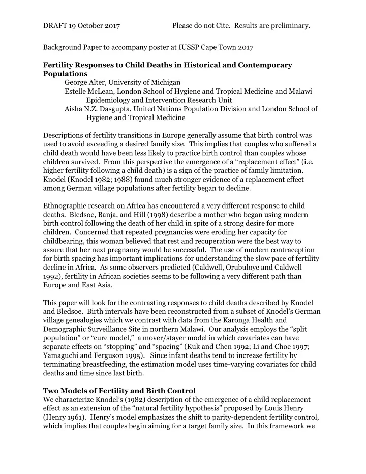
SLIDE 3

DRAFT 19 October 2017 Please do not Cite. Results are preliminary. Karonga HDSS. The total fertility of women in unions decreased from 6.7 in 2002-2007 to 6.1 in 2008-2015. Our regression analysis is limited to women who have had at least one birth, and it is stratified by time period and number of previous births (parity). Tables A3 and A4 show person-years at risk by time period and parity in each sample. We use three time-varying covariates to measure the effect of child deaths on fertility, which are depicted in Figure 1. Breastfeeding reduces fertility by delaying a woman’s return to ovulation. An infant death terminates breastfeeding prematurely and results in an earlier pregnancy, unless the couple is using birth control. To distinguish between the effect of lactation on fertility, we separate the impact of a child death into three periods: 9 to 21, 21 to 33, and 33 to 56 months after the previous birth. If an infant dies, we expect fertility to rise with a nine-month lag. We also expect the impact of lactation to be stronger in the first year after a birth than in the second year. Thus, if an infant dies at age 4 months, we expect fertility to rise 13 months after the birth. We also expect the effect breastfeeding to be greater in the first than in the second year of life. So, we use one variable to measure the effect of ending lactation during the first 12 months of a child’s life (Infant death 1-12 months), and a second variable to measure the effect of ending lactation on fertility during the second year of life (Infant death 13-24 months). In both cases the effect on fertility is lagged by 9 months. Both infant death variables describe effects of the most recent child, and they are reset when another child is born. We use a separate variable (Child death) to measure effects of child deaths that are not related to lactation. To avoid confusing this effect with lactation, this variable takes effect from 33 (i.e. 24+9) to 56 months after the child’s birth, when we expect the impact

• f lactation on fertility to be minimal. Unlike the infant death variables, the child death

variable is not reset after each birth. Since this variable is intended to detect a child replacement effect, the death of the first child should increase motivation for another birth even after the second child is born. Figure 1. Periods Covered by Time-varying Covariates for Child Deaths Months since last birth

0- 2 3- 5 6- 8 9- 11 12- 14 15- 17 18- 20 21- 23 24- 26 27- 29 30- 32 33- 35 36- 38 39- 41 42- 44 45- 47 48- 50 51- 53 54- 56 Infant death 1-12 Infant death 13-24 Child death

SLIDE 4

DRAFT 19 October 2017 Please do not Cite. Results are preliminary. Methods The difference between stopping and spacing can be illustrated by considering survival curves for a birth interval depicted in Figure 2. The birth interval survival curve shows the proportion of women who have not had another birth by time since the last birth. The curve descends rapidly after 9 months, but it tends to level off before reaching 144 months (Casterline and Odden 2016). This means that all of the women who are likely to have another birth have given birth by 144 months, and the women who remain are very unlikely to have another birth. In other words, the proportion who have not had a birth at 144 is a measure of stopping. An increase in the height of the birth interval survival curve at 144 months indicates that the proportion of couples who stopped at that parity has increased. Birth spacing is indicated by the speed of the decrease of the birth interval survival curve from 9 months to its lowest level. If the curve falls more slowly, i.e. it shifts to the right, there will be more long birth intervals and the average length of completed birth intervals will rise. Figure 2. Birth Interval Survival Curves with Stopping and Spacing

SLIDE 5

DRAFT 19 October 2017 Please do not Cite. Results are preliminary. Since birth intervals can change in two distinct ways, we use a statistical model in which covariates can have separate effects on stopping and spacing. The “split-population” or “cure model” has been used most widely in evaluating medical treatments, but there have been some applications in demography (Gray et al. 2010; Kuk and Chen 1992; Li and Choe 1997; Yamaguchi and Ferguson 1995). It provides separate estimates for the proportion who will not experience the transition (stopping, “cured,” “stayers”) and of the timing of those who do make the transition (spacing, “deaths,” “movers”). The proportion of the population surviving at time t is ), ; ( )) ( 1 ( ) ( ) , ; ( z t S x x z x t S

m

     where ) (x  π(x) is the proportion of stayers in the population (also called the “cure fraction” or “stoppers”). The proportion of stayers is modeled by the logistic link function )), exp( 1 /( 1 ) (   x x     where x is a vector of explanatory variables. The survivor function of movers is modeled in the accelerated failure time (AFT) framework with a lognormal function               ' } ln{ 1 ) ; ( z t z t Sm where Φ() is the cumulative distribution for the Gaussian (normal) distribution and z is a vector of explanatory variables. Thus, the model includes two vectors of covariates, x and z, which are used to explain stopping and spacing respectively. Results Estimates from our statistical model are presented in Tables 1 and 2. We are particularly interested in differences between time periods, which show changes during the fertility transitions. We measure changing responses to a child death time by interacting time-period variables with other covariates. Tables 1 and 2 show results for models estimated separately by number of previous children (1-3, 4-6, 7 or more). Covariates appear in both the Stopping and Spacing parts

• f the model. Readers should note that a covariate with a positive estimated

coefficient in the Stopping sub-model increases the proportion who will not have another birth, i.e. more stopping. A positive estimated coefficient in the Spacing sub-model increases the probability of another birth at all durations since the previous birth, which makes birth intervals shorter, i.e. less spacing. The following tables compare predictions from the Natural Fertility Hypothesis and the Bodily Expenditure Hypothesis to our results from the German villages and the Karonga HDSS:

SLIDE 6

DRAFT 19 October 2017 Please do not Cite. Results are preliminary. Predictions and Results of the Natural Fertility Hypothesis Prediction German villages Karonga HDSS Birth spacing played little

• r no role in the fertility

transition.

• Confirmed. Birth intervals

were shorter from 1875 to 1925 than before 1875. Not confirmed. Birth intervals became longer at all parities. The largest increase in spacing was at the lowest parities. Stopping will be most evident at the desired family size. Women with fewer children do not stop. Women with more children are not practicing family limitation.

• Confirmed. Stopping was

least common among women with 7 or more previous births. Not confirmed. Stopping was most common among women with 7 or more previous births. Child replacement will emerge when fertility starts to fall. Partial confirmation. Birth spacing decreased after a death age 2 or older. Not found for stopping. Spacing after deaths under age 2 became shorter. Not confirmed. Birth intervals appear to get longer after a child death, but the results lack statistical significance. Replacement effects should occur among women at the desired family size. Partial confirmation. Spacing after a child death increased most among women with 4-6 previous births. Not confirmed. Infant and child deaths appear to be followed by longer birth intervals. Predictions and Results of the Bodily Expenditure Hypothesis Prediction German villages Karonga HDSS Birth spacing will increase as modern contraception becomes cheaper and more available. Not confirmed. Birth intervals became shorter during the first 50 years of fertility transition. Birth intervals became longer after 1925.

• Confirmed. Birth intervals

became longer at all parities. Birth spacing will be unrelated to number of previous births. Not confirmed. During the fertility transition (1875- 1924) birth spacing became shorter for women with 1-3 or more than 7 previous births. Not confirmed. The largest increase in spacing was at the lowest parities. Stopping will be most common among older (higher parity) women who want to retire from childbearing. Not confirmed. Stopping increased most among women with 1-3 and 4-6 previous births. Partial confirmation. Stopping increase most among women with 4-6 previous births.

SLIDE 7

DRAFT 19 October 2017 Please do not Cite. Results are preliminary. Women will use birth spacing after an infant or child death to regain their

• health. Spacing after an

infant or child death should be more common among older women (higher parities), who need more time to recover their strength. Partially confirmed. Birth intervals following a child (2+ years) death became shorter during the fertility

• transition. Birth intervals

following the death of an infant or 1-year old became

• longer. The increase in

birth intervals after an infant death were greatest at higher parities.

• Confirmed. The largest

increases in birth intervals were among women with more than 7 previous births. Conclusions Fertility decline in Karonga is following a different pattern than the German transition. The German transition began with increases in stopping, but spacing plays a much larger role in Karonga. As Knodel (1982) described, child replacement emerged as fertility declined in Germany. However, child deaths in Karonga may be followed by birth spacing as described in Bledsoe’s work (Bledsoe et al. 1998; Bledsoe and Banja 2002).

SLIDE 8

DRAFT 19 October 2017 Please do not Cite. Results are preliminary.

Table 1. Stopping/Spacing Estimates of Birth Intervals by Number of Previous Births for German Villages 1-3 births 4-6 births 7+ births Coeff. Coeff. Coeff. Stopping sub-model Time period 1700-99

• 0.21
• 0.26

0.22 1800-1849

• 0.63

*

• 0.11
• 0.05

1850-1874 Ref. Ref. Ref. 1875-1899 0.80 ** 0.77 ** 0.43 1900-1924 1.69 ** 1.19 ** 1.10 ** 1925-1950 2.44 ** 2.15 ** 1.43 ** Child death

• 2.56

0.24 0.05 Child death x 1700-99 0.28

• 1.27

0.15 Child death x 1800-1849

• 23.79
• 1.25
• 0.20

Child death x 1850-1874 Ref. Ref. Ref. Child death x 1875-1899

• 17.54
• 0.59

0.13 Child death x 1900-1924 2.03

• 0.25
• 0.33

Child death x 1925-1950 1.42

• 0.18
• 1.59

Spacing sub-model Time period 1700-99

• 0.07

**

• 0.03
• 0.04

1800-1849

• 0.06

**

• 0.07

**

• 0.06

1850-1874 Ref. Ref. Ref. 1875-1899 0.13 ** 0.05 0.15 ** 1900-1924 0.08 ** 0.01 0.10 * 1925-1950

• 0.25

**

• 0.20

** 0.02 Infant death 1-12 months 1.21 ** 1.19 ** 0.99 ** Infant death 1-12 x 1700-99 0.02 0.01 0.20 Infant death 1-12 x 1800-1849 0.14 0.17 0.16 Infant death 1-12 x 1850-1874 Ref. Ref. Ref. Infant death 1-12 x 1875-1899

• 0.04
• 0.26

**

• 0.16

Infant death 1-12 x 1900-1924

• 0.19

*

• 0.24

*

• 0.17

Infant death 1-12 x 1925-1950 0.00 0.04 0.52 Infant death 13-24 months 1.00 ** 0.87 ** 0.91 ** Infant death 13-24 x 1700-99 0.01

• 0.01
• 0.06

Infant death 13-24 x 1800-1849 0.10 0.08

• 0.01

Infant death 13-24 x 1850-1874 Ref. Ref. Ref. Infant death 13-24 x 1875-1899

• 0.22

**

• 0.13
• 0.11

Infant death 13-24 x 1900-1924

• 0.32

**

• 0.14
• 0.25

* Infant death 13-24 x 1925-1950

• 0.16
• 0.10
• 0.12

SLIDE 9

DRAFT 19 October 2017 Please do not Cite. Results are preliminary.

Child death 0.06 0.09 * 0.06 Child death x 1700-99

• 0.07
• 0.15

**

• 0.04

Child death x 1800-1849

• 0.09
• 0.09

0.00 Child death x 1850-1874 Ref. Ref. Ref. Child death x 1875-1899

• 0.08

0.09 0.01 Child death x 1900-1924 0.00 0.10 0.12 Child death x 1925-1950 0.09 0.09

• 0.15

Constant

• 1.22

**

• 1.18

**

• 1.14

** Shape constant 0.60 ** 0.63 ** 0.60 ** LR Chi-squared 7282.77 ** 5767.95 ** 3260.62 ** D.f. 52.00 54.00 51.00 Log likelihood

• 17206.67
• 11521.13
• 6062.46

SLIDE 10

DRAFT 19 October 2017 Please do not Cite. Results are preliminary.

Table 2. Cure Model Estimates of Birth Intervals by Number of Previous Births for Karonga HDSS 1-3 4-6 7+ Coeff. Coeff. Coeff. Stopping sub-model Time period 2002-07 Ref. Ref. Ref. 2008-15 0.05 0.68 ** 0.18 Child death

• 18.33

0.04

• 1.67

Child death x 2002-07 Ref. Ref. Ref. Child death x 2008-15 17.55 0.61 2.32 * Spacing sub-model Time period 2002-07 Ref. Ref. Ref. 2008-15

• 0.12

**

• 0.12

**

• 0.17

** Infant death 1.00 ** 1.20 ** 1.12 ** Infant death x 2002-07 Ref. Ref. Ref. Infant death x 2008-15 0.07

• 0.06

0.13 Death of 1- year old 0.43 ** 0.58 ** 0.50 ** Death 1- yr old x 2002-07 Ref. Ref. Ref. Death 1- yr old x 2008-15

• 0.05

*

• 0.03

0.12 Child death

• 0.09

0.02 0.17 Child death x 2002-07 Ref. Ref. Ref. Child death x 2008-15 0.10 0.10

• 0.07

Polygamous 0.00 0.00 0.04 Constant

• 1.38

**

• 1.35

**

• 1.35

** Shape constant 1.03 ** 0.93 ** 1.02 ** LR Chi-squared 3235.49 ** 1992.61 ** 656.91 ** D.f. 20.00 22.00 20.00 Log likelihood

• 10996.77
• 6451.41
• 1664.28

SLIDE 11

DRAFT 19 October 2017 Please do not Cite. Results are preliminary.

Table A1 Number of Births, Person-years at Risk, and Age-specific Birth Rates for Married Women, German Villages Time Period Age 1700- 1799 1800- 1849 1850- 1874 1875- 1899 1900- 1924 1925- 1950 Number of births 15-19 12 12 3 3 3 4 20-24 501 525 253 281 255 115 25-29 1338 1559 914 1068 877 344 30-34 1478 1800 1073 1160 947 369 35-39 1111 1374 851 891 714 289 40-44 480 646 400 367 277 94 45-49 61 76 48 38 24 13 Person-years at risk 15-19 96.0 71.2 22.4 26.1 22.3 37.2 20-24 1565.3 1522.6 763.9 806.5 803.8 502.0 25-29 3744.1 4096.3 2373.1 2657.2 2608.7 1496.3 30-34 4366.4 4900.7 3038.6 3338.0 3351.9 2129.6 35-39 4064.4 4725.5 2924.9 3284.5 3421.9 2323.2 40-44 3475.9 4201.2 2678.4 3059.0 3367.0 2239.9 45-49 2869.3 3552.6 2273.9 2760.2 3155.6 1998.9 Age-specific birth rates 15-19 0.125 0.169 0.134 0.115 0.134 0.108 20-24 0.320 0.345 0.331 0.348 0.317 0.229 25-29 0.357 0.381 0.385 0.402 0.336 0.230 30-34 0.338 0.367 0.353 0.348 0.283 0.173 35-39 0.273 0.291 0.291 0.271 0.209 0.124 40-44 0.138 0.154 0.149 0.120 0.082 0.042 45-49 0.021 0.021 0.021 0.014 0.008 0.007 TMFR 7.9 8.6 8.3 8.1 6.8 4.6

SLIDE 12

DRAFT 19 October 2017 Please do not Cite. Results are preliminary.

Table A2 Number of Births, Person-years at Risk, and Age-specific Birth Rates for Women in Unions, Karonga HDSS Time Period Age 2002-2007 2008-2015 Number of births 15-19 1191 1786 20-24 1917 2408 25-29 1496 1975 30-34 952 1251 35-39 505 634 40-44 151 175 45-49 14 10 Person-years at risk 15-19 3112.2 4718.4 20-24 5757.2 8490.0 25-29 5858.3 9039.5 30-34 4932.2 7573.8 35-39 3987.5 5570.9 40-44 3885.9 3240.5 45-49 3623.5 1714.8 Age-specific birth rates 15-19 0.383 0.379 20-24 0.333 0.284 25-29 0.255 0.218 30-34 0.193 0.165 35-39 0.127 0.114 40-44 0.039 0.054 45-49 0.004 0.006 TMFR 6.7 6.1

SLIDE 13

DRAFT 19 October 2017 Please do not Cite. Results are preliminary.

Table A3 Person-years at Risk by Age, Time Period and Parity Time Period Age All 1700- 1799 1800- 1849 1850- 1874 1875- 1899 1900- 1924 1925- 1950 1-3 previous births 15-19 275.1 96.0 71.2 22.4 26.1 22.3 37.2 20-24 5828.2 1529.5 1484.6 753.2 787.7 784.0 489.2 25-29 13853.6 3009.7 3236.2 1944.9 2174.6 2123.6 1364.6 30-34 11144.4 2256.4 2267.4 1562.1 1580.4 1877.0 1601.1 35-39 6960.5 1228.4 1264.9 912.5 918.8 1273.3 1362.7 40-44 5328.9 901.2 922.0 617.0 758.0 1057.3 1073.5 45-49 4714.8 800.0 812.1 539.5 688.2 972.5 902.6 4-6 previous births 15-19 0.0 0.0 0.0 0.0 0.0 0.0 0.0 20-24 134.9 35.8 37.1 10.7 18.8 19.6 12.9 25-29 3017.8 721.9 840.8 419.1 457.0 453.5 125.4 30-34 8467.5 1813.6 2228.2 1239.6 1462.7 1253.0 470.5 35-39 8984.3 1940.4 2159.1 1280.4 1449.3 1360.6 794.6 40-44 6726.0 1223.2 1457.7 967.2 1101.8 1073.7 902.4 45-49 5371.4 836.6 1088.8 712.2 976.4 949.7 807.7 7 or more previous births 15-19 0.0 0.0 0.0 0.0 0.0 0.0 0.0 20-24 0.2 0.0 0.0 0.0 0.0 0.2 0.0 25-29 103.4 12.3 19.1 9.1 25.1 31.6 6.3 30-34 1511.5 295.7 405.0 236.5 294.7 221.9 57.7 35-39 4798.8 895.6 1301.4 732.0 916.1 787.8 165.9 40-44 6965.8 1351.3 1821.6 1094.2 1199.2 1235.6 264.1 45-49 6524.3 1232.7 1651.8 1022.2 1095.6 1233.5 288.6

SLIDE 14

DRAFT 19 October 2017 Please do not Cite. Results are preliminary.

Table A4 Person-years at Risk by Age, Time Period and Parity, Karonga HDSS Time Period Age All 2002-2007 2008-2015 1-3 previous births 15-19 4684.0 1694.8 2989.3 20-24 12005.1 4737.6 7267.5 25-29 7788.6 2813.7 4974.8 30-34 2715.6 1094.7 1620.9 35-39 1164.1 524.8 639.3 40-44 645.0 350.6 294.4 45-49 347.0 234.2 112.8 4-6 previous births 15-19 3.7 0.0 3.7 20-24 616.2 277.8 338.4 25-29 5239.9 2118.6 3121.3 30-34 7128.2 2564.4 4563.7 35-39 4383.4 1650.0 2733.4 40-44 2341.3 1294.5 1046.7 45-49 1368.4 916.5 451.9 7 or more previous births 15-19 0.0 0.0 0.0 20-24 3.0 3.0 0.0 25-29 65.3 30.8 34.5 30-34 837.6 325.9 511.8 35-39 2456.4 976.2 1480.2 40-44 2901.1 1457.5 1443.6 45-49 2561.5 1726.9 834.6

SLIDE 15

DRAFT 19 October 2017 Please do not Cite. Results are preliminary.

Table A5 Average Frequency of Infant and Child Death Time-varying Covariates by Time Period and Parity, German Villages Time Period Parity 1700- 1799 1800- 1849 1850- 1874 1875- 1899 1900- 1924 1925- 1950 Infant death 0-12 months 1-3 2.4% 3.5% 3.6% 3.6% 2.7% 1.4% 4-6 2.4% 3.4% 4.0% 3.5% 3.2% 1.7% 7+ 2.7% 3.9% 4.3% 5.1% 3.3% 2.2% Infant death 12-24 months 1-3 0.5% 0.6% 0.5% 0.4% 0.3% 0.2% 4-6 0.5% 0.5% 0.7% 0.6% 0.6% 0.4% 7+ 0.5% 0.6% 0.7% 0.9% 0.6% 0.1% Child death 2-4 years after death 1-3 9.3% 10.5% 10.0% 9.3% 7.5% 5.3% 4-6 23.2% 26.5% 28.3% 29.8% 27.0% 17.2% 7+ 29.0% 33.4% 38.1% 42.7% 34.7% 26.3% Table A6 Average Frequency of Infant and Child Death Time-varying Covariates by Time Period and Parity, Karonga HDSS Time Period Parity 2002-2007 2008-2015 Infant death 0-12 months 1-3 0.5% 0.6% 4-6 0.4% 0.4% 7+ 0.3% 0.4% Infant death 12-24 months 1-3 0.3% 0.1% 4-6 0.1% 0.1% 7+ 0.0% 0.2% Child death 2-4 years after death 1-3 0.5% 2.2% 4-6 1.0% 4.6% 7+ 1.0% 6.4%

SLIDE 16

DRAFT 19 October 2017 Please do not Cite. Results are preliminary. References Baschieri, A., J. Cleland, S. Floyd, A. Dube, A. Msona, A. Molesworth, J.R. Glynn, and N.

• French. 2013. "REPRODUCTIVE PREFERENCES AND CONTRACEPTIVE USE:

A COMPARISON OF MONOGAMOUS AND POLYGAMOUS COUPLES IN NORTHERN MALAWI." Journal Of Biosocial Science 45(2):145-166. Bledsoe, C., F. Banja, and A.G. Hill. 1998. "Reproductive Mishaps and Western Contraception: An African Challenge to Fertility Theory." Population and Development Review 24(1):15-57. Bledsoe, C.H.and F. Banja. 2002. Contingent lives: fertility, time, and aging in West

• Africa. Chicago: University of Chicago Press.

Caldwell, J.C., I.O. Orubuloye, and P. Caldwell. 1992. "Fertility Decline in Africa: A New Type of Transition?" Population and Development Review 18(2):211-242. Casterline, J.B.and C. Odden. 2016. "Trends in Inter-Birth Intervals in Developing Countries 1965-2014." Population and Development Review 42(2):173-+. Crampin, A.C., A. Dube, S. Mboma, A. Price, M. Chihana, A. Jahn, A. Baschieri, A. Molesworth, E. Mwaiyeghele, K. Branson, S. Floyd, N. McGrath, P.E.M. Fine, N. French, J.R. Glynn, and B. Zaba. 2012. "Profile: The Karonga Health and Demographic Surveillance System." International Journal of Epidemiology 41(3):676-685. Gray, E., A. Evans, J. Anderson, and R. Kippen. 2010. "Using Split-Population Models to Examine Predictors of the Probability and Timing of Parity Progression." European Journal of Population-Revue Europeenne De Demographie 26(3):275-295. Henry, L. 1961. "Some data on natural fertility." Eugenics Quarterly 8:81-91. Jahn, A., A.C. Crampin, J.R. Glynn, V. Mwinuka, E. Mwaiyeghele, J. Mwafilaso, K. Branson, N. McGrath, P.E.M. Fine, and B. Zaba. 2007. "Evaluation of a village- informant driven demographic surveillance system in Karonga, Northern Malawi." Demographic Research 16:219-247. Knodel, J. 1982. "Child mortality and reproductive behaviour in German village populations in the past: A micro-level analysis of the replacement effect." Population Studies 36(2):177-200. Knodel, J.and E. van de Walle. 1979. "Lessons from the Past: Policy Implications of Historical Fertility Studies." Population and Development Review 5(2):217-245. Knodel, J.E. 1988. Demographic behavior in the past a study of fourteen German village populations in the eighteenth and nineteenth centuries. Cambridge Cambridgeshire, New York: Cambridge University Press. Kuk, A.Y.C.and C.H. Chen. 1992. "A Mixture Model Combining Logistic-Regression with Proportional Hazards Regression." Biometrika 79(3):531-541. Li, L.and M.K. Choe. 1997. "A mixture model for duration data: Analysis of second births in China." Demography 34(2):189-197. Yamaguchi, K.and L.R. Ferguson. 1995. "The Stopping and Spacing of Childbirths and Their Birth-History Predictors - Rational-Choice Theory and Event-History Analysis." American Sociological Review 60(2):272-298.