
SLIDE 1
1 slide DH QG Currents The CP model CP via rep th pert CFT Conclusions
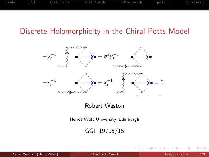
Discrete Holomorphicity in the Chiral Potts Model
Robert Weston
Heriot-Watt University, Edinburgh
GGI, 19/05/15
Robert Weston (Heriot-Watt) DH in the CP model GGI, 19/05/15 1 / 28