
Digital Signal Processing
Markus Kuhn
Computer Laboratory, University of Cambridge https://www.cl.cam.ac.uk/teaching/1920/{DSP,DSP2,L314}/
These notes are provided as an aid for following the lectures, and are not a substitute for attending
Michaelmas 2019 CST Part II(75%)Unit/Part II(50%)/Part III/MPhil ACS
dsp-slides-4up.pdf 2019-11-12 15:52 e67247f 1
Signals
◮ flow of information ◮ measured quantity that varies with time (or position) ◮ electrical signal received from a transducer (microphone, thermometer, accelerometer, antenna, etc.) ◮ electrical signal that controls a process Continuous-time signals: voltage, current, temperature, speed, . . . Discrete-time signals: daily minimum/maximum temperature, lap intervals in races, sampled continuous signals, . . . Electronics (unlike optics) can only deal easily with time-dependent
- signals. Spatial signals, such as images, are typically first converted into
a time signal with a scanning process (TV, fax, etc.).
2
Signal processing
Signals may have to be transformed in order to ◮ amplify or filter out embedded information ◮ detect patterns ◮ prepare the signal to survive a transmission channel ◮ prevent interference with other signals sharing a medium ◮ undo distortions contributed by a transmission channel ◮ compensate for sensor deficiencies ◮ find information encoded in a different domain To do so, we also need ◮ methods to measure, characterise, model and simulate transmission channels ◮ mathematical tools that split common channels and transformations into easily manipulated building blocks
3
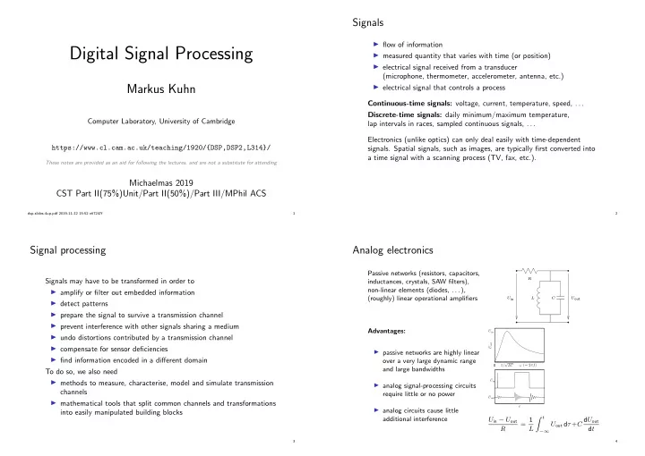
Analog electronics
Passive networks (resistors, capacitors, inductances, crystals, SAW filters), non-linear elements (diodes, . . . ), (roughly) linear operational amplifiers Advantages: ◮ passive networks are highly linear
- ver a very large dynamic range
and large bandwidths ◮ analog signal-processing circuits require little or no power ◮ analog circuits cause little additional interference
R Uin Uout C L ω (= 2πf) Uout 1/ √ LC Uin Uin Uout t
Uin − Uout R = 1 L t
−∞
Uout dτ +C dUout dt
4