Digital Signal Processing for Radio Detection (e.g. of Cosmic Rays) - - PowerPoint PPT Presentation

digital signal processing for radio detection e g of
SMART_READER_LITE
LIVE PREVIEW

Digital Signal Processing for Radio Detection (e.g. of Cosmic Rays) - - PowerPoint PPT Presentation

Digital Signal Processing for Radio Detection (e.g. of Cosmic Rays) KSETA Workshop Roman Hiller, Olga Kambeitz, Dmitriy Kostunin, Dmytro Rogozin | 17.10.2013 K ARLSRUHE I NSTITUTE OF T ECHNOLOGY (KIT) 80 channel 1 60 channel 2 40 Signal (


slide-1
SLIDE 1

KARLSRUHE INSTITUTE OF TECHNOLOGY (KIT)

Digital Signal Processing for Radio Detection (e.g. of Cosmic Rays)

KSETA Workshop Roman Hiller, Olga Kambeitz, Dmitriy Kostunin, Dmytro Rogozin | 17.10.2013

KIT – University of the State of Baden-Wuerttemberg and National Laboratory of the Helmholtz Association

www.kit.edu

  • 80
  • 60
  • 40
  • 20

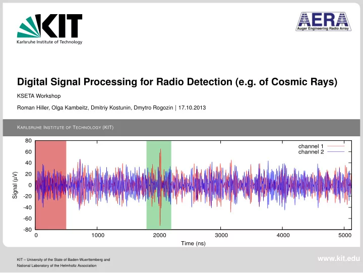
20 40 60 80 1000 2000 3000 4000 5000 Signal (µV) Time (ns) channel 1 channel 2

slide-2
SLIDE 2

Cosmic Rays

  • T. Huege

Cosmic Rays Radio Emission Roman Hiller, Olga Kambeitz, Dmitriy Kostunin, Dmytro Rogozin – Digital Signal Processing for Radio Detection (e.g. of Cosmic Rays)17.10.2013 2/9

slide-3
SLIDE 3

Cosmic Rays

What are they made of? 87 % protons 12 % He nuclei 1 % heavy nuclei

Cosmic Rays Radio Emission Roman Hiller, Olga Kambeitz, Dmitriy Kostunin, Dmytro Rogozin – Digital Signal Processing for Radio Detection (e.g. of Cosmic Rays)17.10.2013 3/9

slide-4
SLIDE 4

Cosmic Rays RADIO

  • R. Engel

Cosmic Rays Radio Emission Roman Hiller, Olga Kambeitz, Dmitriy Kostunin, Dmytro Rogozin – Digital Signal Processing for Radio Detection (e.g. of Cosmic Rays)17.10.2013 4/9

slide-5
SLIDE 5

Cosmic Rays

Cosmic Rays Radio Emission Roman Hiller, Olga Kambeitz, Dmitriy Kostunin, Dmytro Rogozin – Digital Signal Processing for Radio Detection (e.g. of Cosmic Rays)17.10.2013 5/9

slide-6
SLIDE 6

Cosmic Rays

Cosmic Rays Radio Emission Roman Hiller, Olga Kambeitz, Dmitriy Kostunin, Dmytro Rogozin – Digital Signal Processing for Radio Detection (e.g. of Cosmic Rays)17.10.2013 6/9

slide-7
SLIDE 7

Radio Emission

2002 2003 2004 2005 2006 2007 2008 2009 2010 2011 … … LOPES CODALEMA TREND Prototypes at Auger YAKUTSK

[T. Huege] Cosmic Rays Radio Emission Roman Hiller, Olga Kambeitz, Dmitriy Kostunin, Dmytro Rogozin – Digital Signal Processing for Radio Detection (e.g. of Cosmic Rays)17.10.2013 7/9

slide-8
SLIDE 8

Radio Emission

2010 2011 2012 2013 AERA LOFAR Tunka-REX

[T. Huege] Cosmic Rays Radio Emission Roman Hiller, Olga Kambeitz, Dmitriy Kostunin, Dmytro Rogozin – Digital Signal Processing for Radio Detection (e.g. of Cosmic Rays)17.10.2013 8/9

slide-9
SLIDE 9

Radio emission from air showers

Coherent emission at MHz frequencies Two relevant emission mechanisms:

Geomagnetic effect Askaryan effect

  • H. Schoorlemmer K.D. de Vries

Induction of time-varying current Dominant process Time-varying net charge of shower Relative strength: 14 %

Cosmic Rays Radio Emission Roman Hiller, Olga Kambeitz, Dmitriy Kostunin, Dmytro Rogozin – Digital Signal Processing for Radio Detection (e.g. of Cosmic Rays)17.10.2013 9/9

slide-10
SLIDE 10

Roman Hiller, Olga Kambeitz, Dmitriy Kostunin, Dmytro Rogozin – Digital signal processing for Radio Detetction - e.g.of Cosmic Rays 17.10.2013

Propagation and detection of radio emission

Vertical 1017 eV proton-induced air shower at the site of the Pierre Auger

Tim Huege

slide-11
SLIDE 11

Roman Hiller, Olga Kambeitz, Dmitriy Kostunin, Dmytro Rogozin – Digital signal processing for Radio Detetction - e.g.of Cosmic Rays 17.10.2013

Propagation and detection of radio emission

slide-12
SLIDE 12

Roman Hiller, Olga Kambeitz, Dmitriy Kostunin, Dmytro Rogozin – Digital signal processing for Radio Detetction - e.g.of Cosmic Rays 17.10.2013

Propagation and detection of radio emission

Auger Youngsters Meeting 2013, Kathrin Reibelt

slide-13
SLIDE 13

Roman Hiller, Olga Kambeitz, Dmitriy Kostunin, Dmytro Rogozin – Digital signal processing for Radio Detetction - e.g.of Cosmic Rays 17.10.2013

Propagation and detection of radio emission

slide-14
SLIDE 14

Roman Hiller, Olga Kambeitz, Dmitriy Kostunin, Dmytro Rogozin – Digital signal processing for Radio Detetction - e.g.of Cosmic Rays 17.10.2013

Fourier transform

The Scientist and Engineer's Guide to Digital Signal Processing By Steven W. Smith, Ph.D.

slide-15
SLIDE 15

Roman Hiller, Olga Kambeitz, Dmitriy Kostunin, Dmytro Rogozin – Digital signal processing for Radio Detetction - e.g.of Cosmic Rays 17.10.2013

Fourier transform Forward Discrete Fourier Transform: Inverse Discrete Fourier Transform: Amplitude and phase respectively are:

  

1 / 2

] [ ] [

N n N kn i

e i x k X

 

1 / 2

] [ 1 ] [

N k N kn i

e k X N n x

N k X k X N k X

/ ) ]) [ Im( ]) [ Re( / ] [

2 2 

         ] [ Re ] [ Im arctan ]) [ arg(

k X k X k X

slide-16
SLIDE 16

Roman Hiller, Olga Kambeitz, Dmitriy Kostunin, Dmytro Rogozin – Digital signal processing for Radio Detetction - e.g.of Cosmic Rays 17.10.2013

Fourier transform

The Scientist and Engineer's Guide to Digital Signal Processing By Steven W. Smith, Ph.D.

slide-17
SLIDE 17

Roman Hiller, Olga Kambeitz, Dmitriy Kostunin, Dmytro Rogozin – Digital signal processing for Radio Detetction - e.g.of Cosmic Rays 17.10.2013

Fourier transform

The Scientist and Engineer's Guide to Digital Signal Processing By Steven W. Smith, Ph.D.

slide-18
SLIDE 18

Roman Hiller, Olga Kambeitz, Dmitriy Kostunin, Dmytro Rogozin – Digital signal processing for Radio Detetction - e.g.of Cosmic Rays 17.10.2013

Fourier transform

The Scientist and Engineer's Guide to Digital Signal Processing By Steven W. Smith, Ph.D.

slide-19
SLIDE 19

Roman Hiller, Olga Kambeitz, Dmitriy Kostunin, Dmytro Rogozin – Digital signal processing for Radio Detetction - e.g.of Cosmic Rays 17.10.2013

Fourier transform

The Scientist and Engineer's Guide to Digital Signal Processing By Steven W. Smith, Ph.D.

slide-20
SLIDE 20

Roman Hiller, Olga Kambeitz, Dmitriy Kostunin, Dmytro Rogozin – Digital signal processing for Radio Detetction - e.g.of Cosmic Rays 17.10.2013

Fourier transform

The Scientist and Engineer's Guide to Digital Signal Processing By Steven W. Smith, Ph.D.

slide-21
SLIDE 21

Roman Hiller, Olga Kambeitz, Dmitriy Kostunin, Dmytro Rogozin – Digital signal processing for Radio Detetction - e.g.of Cosmic Rays 17.10.2013

Fourier transform

The Scientist and Engineer's Guide to Digital Signal Processing By Steven W. Smith, Ph.D.

slide-22
SLIDE 22

Roman Hiller, Olga Kambeitz, Dmitriy Kostunin, Dmytro Rogozin – Digital signal processing for Radio Detetction - e.g.of Cosmic Rays 17.10.2013

Fourier transform

The Scientist and Engineer's Guide to Digital Signal Processing By Steven W. Smith, Ph.D.

slide-23
SLIDE 23

Roman Hiller, Olga Kambeitz, Dmitriy Kostunin, Dmytro Rogozin – Digital signal processing for Radio Detetction - e.g.of Cosmic Rays 17.10.2013

Fourier transform

The Scientist and Engineer's Guide to Digital Signal Processing By Steven W. Smith, Ph.D.

slide-24
SLIDE 24

Roman Hiller, Olga Kambeitz, Dmitriy Kostunin, Dmytro Rogozin – Digital signal processing for Radio Detetction - e.g.of Cosmic Rays 17.10.2013

Fourier transform

The Scientist and Engineer's Guide to Digital Signal Processing By Steven W. Smith, Ph.D.

slide-25
SLIDE 25

Hardware response

  • Oct. 17th 2012
slide-26
SLIDE 26

Description

  • Oct. 17th 2012

Linearity f(x + y) = f(x) + f(y) and f(ax) = a · f(x)

→ f(sin(ωt)) = α · sin(ωt + ϕ)

S21 = α · eiϕ e.g. from network analyzer

20 40 60 80 100 120 f(MHz) −80 −60 −40 −20 20 40 G(dB)

slide-27
SLIDE 27

Pulse response

  • Oct. 17th 2012

f(MHz) f(MHz)

slide-28
SLIDE 28

Deconvolution

  • Oct. 17th 2012

Linearity → uniqueness Convolution theorem fADC(t) = fin(t) ∗ gfilter(t) fADC(t) ∗ f(t) = F −1(fADC(ν) · gfilter(ν)) reality: cut attenuation region, freal = fin + fN

1.6 1.8 2.0 2.2 2.4 t(ns) ×103 −0.05 0.00 0.05 S(V) 1.6 1.8 2.0 2.2 2.4 t(ns) ×103 −0.10 −0.05 0.00 0.05 0.10 S(V)

slide-29
SLIDE 29

Digital filtering

slide-30
SLIDE 30

Raw data

0.1 1 10 30 40 50 60 70 80 Signal (µV/MHz) Frequency (MHz) channel 1 channel 2

  • 200
  • 100

100 200 1000 2000 3000 4000 5000 Signal (µV) Time (ns) channel 1 channel 2

slide-31
SLIDE 31

Median filter

0.1 1 10 30 40 50 60 70 80 Signal (µV/MHz) Frequency (MHz) channel 1 channel 2

  • 200
  • 100

100 200 1000 2000 3000 4000 5000 Signal (µV) Time (ns) channel 1 channel 2

slide-32
SLIDE 32

Bandstop filter

0.1 1 10 30 40 50 60 70 80 Signal (µV/MHz) Frequency (MHz) channel 1 channel 2

  • 200
  • 100

100 200 1000 2000 3000 4000 5000 Signal (µV) Time (ns) channel 1 channel 2 SNR=12.8 !!!

slide-33
SLIDE 33

Exercise 1

  • Oct. 17th 2012

Draw a Low Pass Filter in frequency and time domain. Explain how it works in frequency/time domain?

slide-34
SLIDE 34

Exercise 1

  • Oct. 17th 2012

Fre que ncy

a . Low-pa ss

passband stopband transition band

Am plitude

S

10 20 30

  • 0.02

0.00 0.02 0.04 0.06 0.08

Sample number

Amplitude

slide-35
SLIDE 35

Exercise 2

  • Oct. 17th 2012

Draw a High Pass filter in frequency and time domain. Tipp: For the time domain use the linearity of the fourier transform to derive the high pass from known spectra (low pass and ?). Explain how it works in frequency/time domain?

slide-36
SLIDE 36

Exercise 2

  • Oct. 17th 2012

Fre que ncy

  • b. High-pa

ss

Am plitude

S

10 20 30

  • 0.25

0.00 0.25 0.50 0.75 1.00 1.25

Sample number

Amplitude

slide-37
SLIDE 37

Exercise 3

  • Oct. 17th 2012

Explain, why both signals have the same spectrum.

20 40 60 80 100 f(MHz) 10
  • 3
10
  • 2
10
  • 1
10 10 1 10 2 1000 2000 3000 4000 5000 6000 t(ns) 0.2 0.1 0.0 0.1 0.2 0.3 0.4 0.5 1000 2000 3000 4000 5000 6000 t(ns) 0.10 0.08 0.06 0.04 0.02 0.00 0.02 0.04 0.06 0.08

FFT

slide-38
SLIDE 38

Exercise 3

  • Oct. 17th 2012
1000 2000 3000 4000 5000 6000 t(ns) 0.2 0.1 0.0 0.1 0.2 0.3 0.4 0.5 1000 2000 3000 4000 5000 6000 t(ns) 0.10 0.08 0.06 0.04 0.02 0.00 0.02 0.04 0.06 0.08 20 40 60 80 100 1 2 3 4 5 6 7

f(MHz)

20 40 60 80 100 100 200 300 400 500 600

f(MHz)

Phases

slide-39
SLIDE 39

Exercise 4

  • Oct. 17th 2012

kseta.boson.su