Detailed Routing Find actual geometric layout of each Global Routing - - PDF document

11/2/2018 1

DET A IL ED RO UT ING

PRO F. INDRA NIL SENG UPT A

DEPA RT MENT O F C O MPUT ER SC IENC E A ND ENG INEERING DEPA RT MENT O F C O MPUT ER SC IENC E A ND ENG INEERING

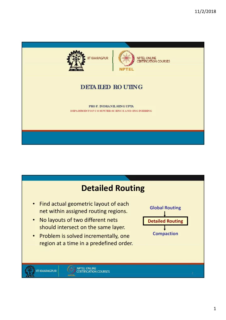
Detailed Routing

• Find actual geometric layout of each

i hi i d i i

Global Routing

net within assigned routing regions.

• No layouts of two different nets

should intersect on the same layer.

• Problem is solved incrementally, one

region at a time in a predefined order

Detailed Routing G oba

• ut g

Compaction

2

region at a time in a predefined order.

11/2/2018 2

A Routing Example

3

Placement Global Routing Detailed Routing

After Global Routing

• The two‐stage routing method is a powerful technique for

ti routing.

• During the global routing stage:

– The routing region is partitioned into a collection of rectangular regions. – To interconnect each net, a sequence of sub‐regions to be used is determined. – All nets crossing a given boundary of a routing region are called floating l

4

terminals. – Once the sub‐region is routed, these floating terminals become fixed terminals for subsequent regions.

11/2/2018 3

Channels and Switchboxes

• There are normally two kinds of rectilinear regions.

– Channels: routing regions having two parallel rows of fixed terminals. – Switchboxes: generalizations of channels that allow fixed terminals on all four sides of the region.

Channel

5

Channel Switchbox

Order of Routing Regions

• Slicing placement topology.

– Nets can be routed by considering

1

– Nets can be routed by considering channels 1, 2 and 3 in order.

• Non‐slicing placement topology.

– Channels with cyclic constraints

4 1 3 2

6

Channels with cyclic constraints. – Some of the routing regions are to be considered as switchboxes.

3 2

11/2/2018 4

Routing Considerations

• Number of terminals

– Majority of nets are two terminal ones – Majority of nets are two‐terminal ones. – For some nets (viz. clock, power), number of terminals can be very large. – Each multi‐terminal net can be decomposed into several two‐terminal nets.

• Net width

– Power and ground nets have greater width. – Signal nets have less width

7

Signal nets have less width.

• Via restrictions

– Regular: only between adjacent layers. – Stacked: passing through more than two layers.

• Boundary type

– Regular: straight border of routing region – Irregular: arbitrary

• Number of layers

– Modern fabrication technology allows at least five layers of routing.

8

• Net types

– Critical: power, ground, clock nets – Non‐critical: signal nets

11/2/2018 5

CMOS Fabrication

9

Via Connections

10

11/2/2018 6

Routing Models

• Grid‐based model

– A grid is super‐imposed on the A grid is super imposed on the routing region. – Wires follow paths along the grid lines.

• Gridless model

11

– Does not follow the gridded approach.

Models for Multi‐Layer Routing

• Unreserved layer model

– Any net segment is allowed to be placed in any layer.

• Reserved layer model

– Certain types of segments are restricted to particular layer(s).

T l (HV VH)

12

• Two‐layer (HV, VH)
• Three‐layer (VHV, HVH)

11/2/2018 7

Illustration

HVH Model VHV Model Layer 1

13

Unreserved Layer Model Layer 2 Layer 3

Channel Routing

• In channel routing, interconnections are made within a

rectangular region having no obstructions.

– A majority of modern‐day ASICs use channel routers. – Algorithms are efficient and simple. – Guarantees 100% completion if channel width is adjustable.

14

11/2/2018 8

• Some terminologies:

– Track: horizontal row available for routing. – Trunk: horizontal wire segment. – Branch: vertical wire segment connecting trunks to terminals. – Via: connection between a branch and a trunk.

15

Channel Routing Problem :: Terminologies

2 2 1 3 Upper boundary 1 1 3 3 Lower boundary Net list:: TOP = [ 1 2 0 2 3 ] [ ] 2 2 1 3

16

BOT = [ 3 3 1 1 0 ] 1 1 3 3

11/2/2018 9

Problem Formulation

• The channel is defined by a rectangular region with

two rows of terminals along its top and bottom sides.

– Each terminal is assigned a number between 0 and N. – Terminals having the same label i belong to the same net i. – A ‘0’ indicates no connection

17

A 0 indicates no connection.

• The task of the channel router is to:

– Assign horizontal segments of nets to tracks Assign horizontal segments of nets to tracks. – Assign vertical segments to connect

a) Horizontal segments of the same net in different tracks. b) The terminals of the net to horizontal segments of the net.

• Channel height should be minimized.

18

Channel height should be minimized.

• Horizontal and vertical constraints must be met.

11/2/2018 10

Channel Constraints

• Horizontal constraints between two nets:

– The horizontal span of two nets overlaps each other. – The nets must be assigned to separate tracks.

• Vertical constraints between two nets:

– There exists a column such that the terminal i on top of the column belongs to one net and the terminal j on bottom of the

19

column belongs to one net, and the terminal j on bottom of the column belongs to the other net. – Net i must be assigned a track above that for net j.

Horizontal Constraint Graph (HCG)

• It is a graph where vertices represent nets, and edges

represent horizontal constraints.

1 1 2 2 5 1 4 3 1 2 5 4

20

3 2 1 3 4 3 5 2 3 4

11/2/2018 11

Vertical Constraint Graph (VCG)

• It is a directed graph where vertices represent nets, and

edges represent vertical constraints.

4 3 1 1 2 2 5 1 1 4 2

21

3 4 3 5 2 1 3 2 5 3

Two‐layer Channel Routing

• Left‐Edge Algorithms (LEA)

– Basic Left‐Edge Algorithm asic eft dge Algorithm – Left‐Edge Algorithm with Vertical Constraints – Dogleg Router

• Constraint‐Graph Based Algorithm

– Net Merge Channel Router

• Greedy Channel Router

22

• Greedy Channel Router
• Hierarchical Channel Router

11/2/2018 12

Basic Left Edge Algorithm

• Simplest channel routing algorithm.

A i

• Assumptions:

– Only two‐terminal nets. – No vertical constraints. – HV two‐layer model.

23

– Doglegs are not allowed.

• Basic Steps:

– Sort the nets according to the x‐coordinate of the leftmost terminal of the net. – Route the nets one‐by‐one according to the order. – For a net, scan the tracks from top to bottom, and assign it to the first track that can accommodate it.

• In the absence of vertical constraints, the algorithm

produces a minimum‐track solution.

24

11/2/2018 13

Extension to Left‐Edge Algorithm

• Vertical constraints may exist, but there are no directed cycles in the VCG.
• Select a net for routing if both the following conditions are true:

a) The x‐coordinate of the leftmost terminal is the least. b) There is no edge incident on the vertex corresponding to that net in the VCG.

• After routing a net, the corresponding vertex and the incident edges are

deleted from the VCG.

25

• Other considerations are the same as the basic left‐edge algorithm.

5 7 4 5 2 4 1 1 8 7 6 8 6 3 3 2 1 3 8 7

26

2 8 7 6 5

VCG

11/2/2018 14 5 7 4 5 2 4 1 1 8 7 6 8 6 3 3 2 1 3 8 7

27

2 8 7 6 5

VCG

5 7 4 5 2 4 1 1 8 7 6 8 6 3 3 2 1 3 8 7

28

2 8 7 6 5

VCG

11/2/2018 15 5 7 4 5 2 4 1 1 8 7 6 8 6 3 3 2 1 3 8 7

29

2 8 7 6 5

VCG

5 7 4 5 2 4 1 1 8 7 6 8 6 3 3 2 1 3 8 7

30

2 8 7 6 5

VCG

11/2/2018 16

Dogleg Router

• Drawback of LEA:

The entire net is on a single track – The entire net is on a single track. – Sometimes leads to routing with more tracks than necessary.

• Doglegs are used to place parts of the same net on different

tracks.

– A dogleg is a vertical segment that connects two trunks located in two

31

g g g different tracks. – May lead to a reduction in channel height.

• Dogleg router allows multi‐terminal nets and vertical

constraints.

– Multi‐terminal nets are broken into a series of two‐terminal nets.

• Cannot handle cyclic vertical constraints.

32

11/2/2018 17

Dogleg Example

2 3 2 1 1 2 3 2 1 1 3 3 2 3 2 3

33

3 3 2 3 2 3

No dogleg 3 tracks With dogleg 2 tracks

Dogleg Router: Algorithm

• Step 1:

f l h h f l – If cycle exists in the VCG, return with failure.

• Step 2:

– Split each multi‐terminal net into a sequence of 2‐terminal nets.

• A net 2 .. 2 .. 2 will get broken as 2a .. 2a 2b .. 2b.

– HCG and VCG gets modified accordingly.

34

• Step 3:

– Apply the extended left‐edge algorithm to the modified problem.

11/2/2018 18

3 4 2 2 1 1 3 2 4 4 4 3 3 2 1 4 3b 4a 2b 2a 2b 1

1 2a

35

4b 4a 4b 3a 3b 3a 2a 1

2b 3a 4a 3b

3b 4a 2b 2a 2b 1 1 2b 4b 4a

1 2a 2b 3a 4a 3b

36

4b 4a 4b 3a 3b 3a 2a 1

11/2/2018 19

3b 4a 2b 2a 2b 1 1 2a 2b 3a 3b 4b 4a

37

4b 4a 4b 3a 3b 3a 2a 1

Net Merge Channel Router

• Due to Yoshimura and Kuh.
• Basic idea:

– If there is a path of length p in the VCG, at least p horizontal tracks are required to route the channel. – Try to minimize the longest path in the VCG.

38

– Merge nodes of VCG to achieve this goal.

• Does not allow doglegs or cycles in the VCG.

11/2/2018 20

How does it work?

• Partition the routing channel into a number of regions

called zones.

• Nets from adjacent zones are merged.

– Merged nets are treated as a composite net and assigned to a single track.

39

Key Steps of the Algorithm

a) Zone representation b) Net merging c) Track assignment 10 9 4 7 6 1 5 4 1 10

40

7 9 8 6 2 5 3 5 3 2 8 9

11/2/2018 21

Step 1: Zone Representation

• Let S(i) denote the set of nets whose horizontal segments

i l i intersect column i.

• Take only those S(i) which are maximal, that is, not a

proper subset of some other S(j).

• Define a zone for each of the maximal sets.

I t f HCG / i t l h d t

41

• In terms of HCG / interval graph, a zone corresponds to a

maximal clique in the graph.

Column S(i) Zone 1 {2} 2 {1,2,3} 3 {1,2,3,4,5} 1 4 {1,2,3,4,5}

Z1 Z2 Z3 Z4 Z5

1 7 2 8 3 9 10 4 Zone presentation

{ } 5 {1,2,4,5} 6 {2,4,6} 2 7 {4,6,7} 3 8 {4,7,8} 9 {4,7,8,9} 4 10 {7,8,9} 11 {7 9 10} 5

6 10 4 5 Rep

7 5 9 4 1 10

42

11 {7,9,10} 5 12 {9,10}

Zone Table

3 8 2 6 VCG

11/2/2018 22

Step 2: Net Merging

• Let Ni and Nj be two nets for which the following conditions are

satisfied: satisfied:

– There is no edge between vi and vj in HCG. – There is no directed path between vi and vj in VCG.

• Nets Ni and Nj can be merged to form a new composite net.

– Modifies VCG by merging nodes vi and vj into a single node vi.j.

43

– Modifies HCG / zone representation by replacing nodes vi and vj by a net vi‐j, which occupies the consecutive zones including those of nets Ni and Nj.

• The process is iterative:

P i f d i l d – Pairs of nodes are successively merged. – At every step of the iteration, in case of multiple choices, merge the net‐pair that minimizes the length of the longest path in the VCG. – That is, the increase in length is minimum.

• A result:

44

– If the original VCG has no cycles, then the updated VCG with merged nodes will not have cycles either.

11/2/2018 23

• Iteration 1 of the example:

– We can merge nets pairs (1,6), (3,6) or (5,6).

3 7 5 9 4 8 2 1.6 10 4 1 10 3.6 7 5 9 4 8 1 10

Best Choice

45

2 3 7 5.6 9 8 2 2

• Successive iteration steps:

10 10 3 9 4 8 2 1.7 5.6 4 1.7 5.6.9 2 3 8 1.7 5.6.9 4.10

46

2 3.8 3.8 2

11/2/2018 24

Step 3: Track Assignment

• Each node in the final graph is assigned a separate track.
• Actually we apply the left‐edge algorithm to assign horizontal tracks to the merged

y pp y g g g g nets. – The list of nets sorted on their left edges, subject to the vertical constraint, is: [ 4‐10, 1‐7, 5‐6‐9, 2, 3‐8 ]

Track 1: Nets 4 and 10 Track 2: Nets 1 and 7

47

Track 3: Nets 5, 6 and 9 Track 4: Net 2 Track 5: Nets 3 and 8

The Final Solution

10 9 4 7 6 1 5 4 1 10

48

7 9 8 6 2 5 3 5 3 2 8 9

11/2/2018 25

Greedy Channel Router

• The routing algorithms discussed so far route the channel one net at a

time time.

– Based on left‐edge algorithm or some of its variation.

• The Greedy Channel Router algorithm routes the channel column by

column starting from the left.

– Apply a sequence of greedy but intelligent heuristic at each column. – Objective is to maximize the number of tracks available in the next column.

49

j

• Can handle problems with cycles in VCG.

– May need additional columns at the end of the channel.

• Some of the heuristics used:

– Place all segments column by column, starting from the leftmost column. – Connect any terminal to the trunk segment of the corresponding net. – Collapse any split net using a vertical segment. – Try to reduce the distance between two tracks of same net. – Try to move the nets closer to the boundary which contains the next terminal

50

• f that net.

– Add additional tracks if needed.

11/2/2018 26

Channel Routed using a Greedy Router

1 2 3 1 3 2 1 4 3

51

2 4 3 1 2 3 4 5 5

Comparison of Two‐Layer Channel Routers

LEA Dogleg Net Merge Greedy Model Grid-based Grid-based Grid-based Grid-based Dogleg No Yes Yes Yes Vertical constraint No / Yes Yes Yes Yes Cyclic constraint No No No Yes

52

Cyclic constraint No No No Yes

11/2/2018 27

• Several approaches:

Three‐Layer Channel Routing

pp

– Extended Net Merge Channel Router – HVH Routing from HV Solution – Hybrid HVH‐VHV Router

53

HVH Routing from HV Solution

• Very similar to the Y‐K algorithm.

– Systematically transform a two layer routing solution into a three layer – Systematically transform a two‐layer routing solution into a three‐layer routing solution. – In Y‐K algorithm, nets are merged so that all merged nets forming a composite net are assigned to one track. – Here, the composite nets are merged to form super‐composite nets.

• Objective:

54

• Objective:

– Reduce the number of super‐composite nets.

11/2/2018 28

• Two composite nets in a super‐composite net can be assigned

to different layers on the same track.

• A track‐ordering graph is used to find the optimal pair of

A track ordering graph is used to find the optimal pair of composite nets to be merged.

– Vertices represent the composite (tracks) in a given two‐layer solution. – The directed edges represent the ordering restrictions on pairs of tracks.

55

• Composite interval ti must be routed above composite interval tj, if there

exists a net Npti and Nqtj, such that Np and Nq have a vertical constraint. Track ordering graph

56

11/2/2018 29

An optimal scheduling solution Graph representation

57

Switchbox Routing

• A switchbox is a generalization of a channel.

Has terminals on all four sides – Has terminals on all four sides.

• More difficult than channel routing problem.

– Main objective of channel routing is to minimize the channel height. – Main objective of switchbox routing is to ensure that all the nets are routed.

• Classification of algorithms:

– Greedy router

58

Greedy router – Rip up and reroute routers – BEAVER (based on computational geometry)

11/2/2018 30

59

Summary

• The detailed routing problem is solved by routing the channels and

switchboxes.

• Routing results may differ based on the routing model used.

– Grid‐based. – Based on assigning layer of different net segments.

• The objectives for routing a channel is to minimize channel density, the

length of routing nets, and the number of via’s.

60

g g ,

• The main objective of channel routing is to minimize total routing area.
• The objective of switchbox routing is to determine the routability.

11/2/2018 31

Over‐The‐Cell Routing Introduction

• Used in sophisticated channel routers in standard cell

b d d i based designs.

• Basic idea:

– Use of area outside the channel to obtain reduction in channel height. Routing over the cell rows is possible due to limited use of

CAD for VLSI 62

– Routing over the cell rows is possible due to limited use of the second and third metal layers.

11/2/2018 32

Basic Steps in OTC Routing

• Step 1: Net decomposition

Each multi terminal net is partitioned into a set of 2 terminal nets – Each multi‐terminal net is partitioned into a set of 2‐terminal nets (defined based on x‐coordinates of their left ends).

• Step 2: Net classification

– Each net is classified into one of following types:

• Type 1: There is a vacant terminal directly opposite to one of the

terminals of the net.

CAD for VLSI 63

terminals of the net.

• Type 2: There is a vacant terminal between the two terminals of the net.
• Type 3: None of the above.
• Step 3: Vacant terminal assignment

– Vacant terminals are assigned to each net depending on its type and weight. – Weight of a net is defined as the improvement in channel congestion possible if this net can be routed over the cell.

• Step 4: Over‐the‐cell routing

– The selected nets are assigned exact geometric paths for routing in the area over the cells.

• Step 5: Channel segment assignment & routing

– Selects the best net segments to be routed in the channel

CAD for VLSI 64

Selects the best net segments to be routed in the channel. – Route them using any available channel router.

11/2/2018 33

Example

Greedy channel router OTC routing

CAD for VLSI 65

OTC routing