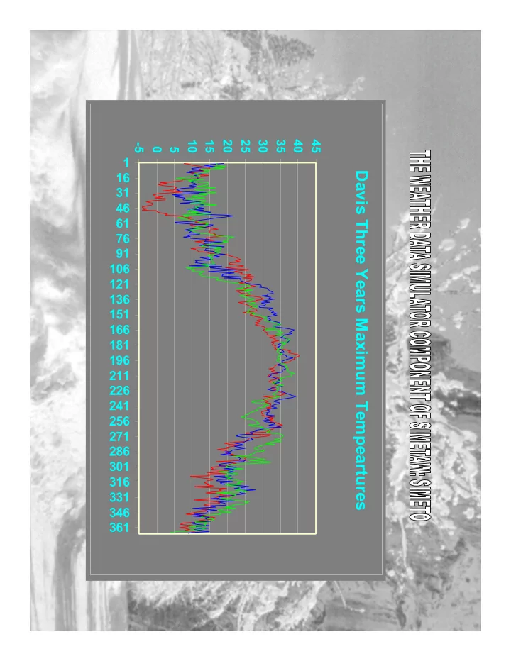
Davis Three Years Maximum Tempeartures 16 31 46 61 76 91 106 - PDF document

10 15 20 25 30 35 40 45 -5 0 5 1 Davis Three Years Maximum Tempeartures 16 31 46 61 76 91 106 121 136 151 166 181 196 211 226 241 256 271 286 301 316 331 346 361

SIMETO A model generates daily weather variables based on monthly summaries Model Development Concerns How many parameters are needed? • Overparameterization – Information over-use; inefficient model; unstable model • Underparameterization – Information underutilization; potentially large systematic errors

Basic Data Inputs latitudes, longitudes, elevations (m.) The meteorological variables (a) fractions of wet days (b) rain per wet day (c) maximum temperature (d) minimum temperature (e) solar radiation (f) vapor pressure (g) maximum relative humidity (h) minimum relative humidity (i) wind speed

SIMULATION OF ETo The equations used to simulate reference evapotranspiration (ET0) are taken from R.L. Snyder and W.O. Pruitt (1994) and include the following : (1) Original Penman (2) Penman/Monteith (as used in the FAO CROPWAT program) (3) Corrected FAO Penman (4) Priestley/Taylor (5) Jensen/Haise (6) FAO Radiation (7) FAO Blaney/Criddle (8) SCS Blaney Criddle (9) Hargreaves (10) Corrected FAO evaporation pan

Required Meteorological Data For Eto Calculations Eto Estimate MaxT MinT Solar Humidity Wind EPEN X X X X X PENM X X X X X CFAO X X X X X FAORD X X X X X FAOBC X X X X X EPT X X X X EJH X X X SCSBC X X HARG X X

– Tow Stage Markov Chain: useful to describe time series events • to determine the rain or dry day – Gamma function: a skewed distribution ideal for describe rainfall amount • to determine the amount of rain

Yesterday Wet Dry Today Today Wet Dry wet Dry f 11 (t) 1 f 01 (t) 1 f 10 (t) 1 f 00 (t) 1 P 11 = SUM(f 11 ); P 01 = 1 - P 11; P 10 = SUM(f 10 ); P 00 = 1 - P 10 How many parameters are needed?

A linear relationship exists between the transitional probability and the marginal probability P(W/D) = 0.006 + 0.75 (fraction of wet days); r 2 = 0.96 = 0.75 * (fraction of the wet days) P(W/W) = (1 - b) + b*(Fraction of wet days) = 0.25 + P(W/D) Thus all transitional probability are estimable form the fraction of wet days!

The Amount of Rainfall: Gamma Function Alfa = (0.5000876 + 0.16488552Y -0.0544274Y 2 ) / Y Bata = Arithmetic Mean / Alfa where Y = In(Arithmetic Mean/Geometric Mean)

Alfa < 1 ; unit less; most influential to small numbers Bata has the same unit as the variable and affects extreme numbers, or the tail distribution more than Alfa Thus Bata related to mean more than Alfa?

A Linear Relationship is Established Between Bata and the Mean Amount of Rainfall Per wet day Bata = - 2.16 + 1.83*(amount of rain per wet day) r 2 = 0.965 (0.275) (0.036) Alfa = (Amount per Wet Day) / Bata Thus, given amount rainfall per wet day, we can obtain both Alfa and Bata for the Gamma model to generate rainfall

Other weather Variables: Temperature and Solar Radiation b a Mean Curve = a + b COS [2(Pi)(j - q) /365] where j is Julian day; q is the day with the maximal value X = Mean* ( 1+ d*CV)

CV is the coefficient of variation. “d” measures the influence of other correlated weather variables, the serial correlations, and a random component. d i = B 0 d i-1 + B 1 e i B 0 = R 1 R 0 -1 ’ = R 0 - R 1 R 0 -1 R 1 B 1 B 1 ’ R 0 is the cross correlation matrix , and R 1 is the serial correlation matrix.

1 r 12 r 13 r 21 1 r 23 R 0 = r 31 r 32 1 r ij is the cross correlation between ith and jth variables. r (11) r (12) r (13) r (21) r (22) r (23) R 1 = r (31) r (32) r (33) r (ij) is the serial correlation between ith and jth variable, with the second vraiable lagged one day.

Temperature Curve CV Curve Tmax(CV) = (0.536 - 0.00573 a 0 ) - exp(-4.63 + 0.0952 b) *(COS(2(i-q)/365) Tmin(CV) = exp(-0.0466a) - exp(-4.64 + 0.146b) *COS(2(i-q)/365)

Davis Tmim Raw Data Davis: Observed versus Simulated Daily Tmin 18 18 300 16 16 250 Mean Curve R 2 = 0.93 14 R 2 = 0.82 14 Simulated Tmin 12 12 200 C Degree 10 CV (%) 10 150 8 8 6 6 100 4 4 CV R 2 = 0.71 2 50 2 0 0 0 0 5 10 15 20 1 31 61 91 121 151 181 211 241 271 301 331 361 Observed Tmin Davis Tmin Daily Raw versus Simulated CVs Davis: Raw and Simulated daily Tmin means 18 300 16 250 14 Blue- Raw ;R 2 = 0.71 200 Percent CV 12 10 Red - Simulated ;R 2 = 0.69 150 2 = 0.93 Red -Raw; R 8 100 6 2 = 0.96 Blue -Simulated; R 50 4 2 0 0 0 30 60 90 120 150 180 210 240 270 300 330 360 0 20 40 60 80 100 120 140 160 180 200 220 240 260 280 300 320 340 360 Days in Year

Davis Tmax Raw Data Davis: Observed versus Simulated Daily Tmax 40 60 40 35 35 50 R 2 = 0.96 R 2 = 0.94 30 Simulated Tmax 30 25 40 25 C Degree CV (%) 20 20 30 15 15 10 R 2 = 0.49 20 5 10 10 0 5 0 5 10 15 20 25 30 35 40 0 0 Observed Tmax 1 31 61 91 121 151 181 211 241 271 301 331 361 Davis Tmax Daily Raw versus Simulated CVs Davis: Raw and Simulated daily Tmax means 60 40 Red - Simulated; R 2 = 0.79 50 35 30 Blue - raw; R 2 = 0.49 40 Percent CV 25 30 Red - Simulated; R 2 = 0.96 20 20 15 Blue - Raw; R 2 = 0.96 10 10 5 0 0 20 40 60 80 100 120 140 160 180 200 220 240 260 280 300 320 340 360 0 0 20 40 60 80 100 120 140 160 180 200 220 240 260 280 300 320 340 360 Days in Year

Davis Raw data of Salor Radiation: Daily means and CVs Davis Raw versus Simulated Salor Radiation 35 1.2 35 R 2 = 0.96 30 30 1.0 25 25 0.8 simulated 20 20 MJ/m2 CV 0.6 Blue -Means; R 2 = 0.9767 15 15 Red - CV Curve; R 2 = 0.7307 0.4 10 10 0.2 5 5 0.0 0 0 1 15 29 43 57 71 85 99 113 127 141 155 169 183 197 211 225 239 253 267 281 295 309 323 337 351 365 0 5 10 15 20 25 30 35 raw Davis Observed versus Simulated Daily Salor Radiation Davis Raw Versus Simualtred Daily CV of Salor Radiation 35 1.2 30 1.0 25 2 = 0.73 0.8 Blue - Raw; R 20 Solar 2 = 0.69 Red - Simulated; R CV 0.6 15 Red - Simulated; R 2 = 0.98 0.4 Blue -Raw; R 2 = 0.98 10 0.2 5 0 0.0 1 21 41 61 81 101 121 141 161 181 201 221 241 261 281 301 321 341 361 1 21 41 61 81 101 121 141 161 181 201 221 241 261 281 301 321 341 361

Dvais ETO Raw Data Davis: Observed versus Simulated Daily ETo 8 140 9 8 7 120 R 2 = 0.93 7 6 100 6 R 2 = 0.97 Simulated ETo 5 ETO (mm) 80 5 CV (%) 4 4 60 3 3 R 2 = 0.63 40 2 2 20 1 1 0 0 0 0 1 2 3 4 5 6 7 8 1 31 61 91 121 151 181 211 241 271 301 331 361 Observed ETo ETo Daily CVs: Raw versus Simulated values Davis: Raw and Simulated daily ETo means 140 9 120 8 7 100 Raw CV; R 2 = 0.49 Percent CV 6 80 Simulated CV; R 2 = 0.56 5 60 4 Red- Raw; R 2 = 0.97 40 3 Blue - Simulated; R 2 = 0.95 20 2 1 0 0 0 30 60 90 120 150 180 210 240 270 300 330 360 0 20 40 60 80 100 120 140 160 180 200 220 240 260 280 300 320 340 360 Days in Year

Davis Real and Simulated Monthly Rainfall Red: simulated; Blue: real 140 120 100 Rainfall (mm) 80 60 40 20 0 1 2 3 4 5 6 7 8 9 10 11 12 Month Davis Real and Simulated Rainfall Days per Month Red: simulated; Blue: real 8 7 6 5 4 3 2 1 0 1 2 3 4 5 6 7 8 9 10 11 12 Month Davis Real and Simulated Wind Speed (m/s) Red: Simulated; Blue: Real 3.5 3.0 2.5 2.0 1.5 1.0 0.5 0.0 1 2 3 4 5 6 7 8 9 10 11 12 Month