Data visualization and graphics n e w d a t a < - g a - PDF document

An introduction to WS 2019/2020 l i b r a r y ( t i d y r ) Data visualization and graphics n e w d a t a < - g a t h e r ( s t u d e n t s , G r o u p , N u m b e r , 2 : 7 ) What is this line of code doing? Answer: combine columns 2 to 7 of dataset s t u d e n t s into two columns named Group and Number Dr. Noémie Becker Dr. Eliza Argyridou How many Groups are there in dataset s ? t u d e n t s Answer: 6 groups Special thanks to : Dr. Benedikt Holtmann and Dr. Sonja Grath for sharing slides for this lecture What you should know after day 6 Graphics with base R Review: Rearranging and manipulating data Graphics with base R Simple graphics using plotting functions in the graphics package ● Histograms ● Scatterplots ● Base R, installed by default ● Boxplots ● Easy and quick to type Functjon Descriptjon Saving plots hist() Histograms ● Wide variety of functions Graphics with ggplot2 plot() Scatuerplots, etc. boxplot() Box- and whisker plots barplot() Bar- and column charts dotchart() Cleveland dot plots contour Contour of a surface (2D) pie() Circular pie chart … 3 4 What you should know after day 6 Graphics with base R Creating a histogram with hist() Review: Rearranging and manipulating data Example 1: Graphics with base R ● Histograms h i s t ( S p a r r o w s $ T a r s u s ) ● Scatterplots Hist ogra m of Sparrows$Tarsus ● Boxplots 0 Saving plots 0 2 Graphics with ggplot2 0 5 y 1 c n e u q 0 e 0 r F 1 0 5 0 1 9 2 0 2 1 2 2 2 3 2 4 2 5 S p a r r o w s $ T a r s u s 5 6

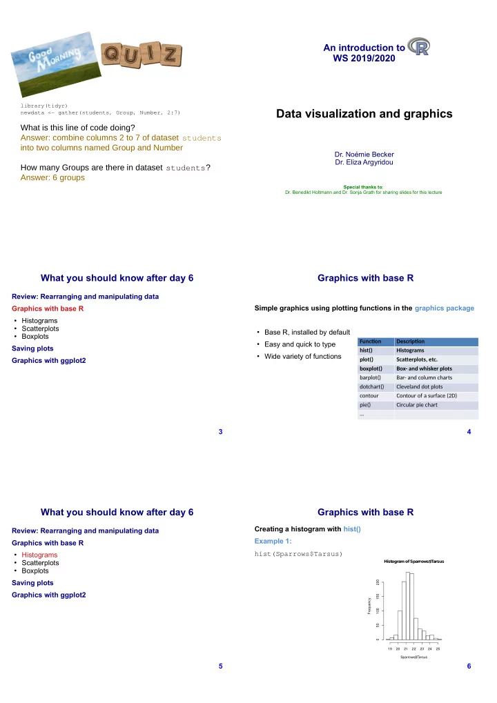
Graphics with base R Graphics with base R Creating a histogram with hist() Creating a histogram with hist() Example 2: Alter colour and the number of bins Example 3: density instead of frequency h i s t ( S p a r r o w s $ T a r s u s , h i s t ( S p a r r o w s $ T a r s u s , Histogram of Sparrows$T arsus Hist ogram of Sparr ow s$ Tarsus c o l = " g r e y " , c o l = " g r e y " , 6 . 0 0 6 b r e a k s = 5 0 , b r e a k s = 5 0 ) 0 5 4 . 0 y f r e q = F A L S E ) t i s 0 4 n e y D c 2 . n e 0 0 3 u q e r F 0 2 0 . 0 0 1 1 9 2 0 2 1 2 2 2 3 2 4 2 5 0 S p a r r o w s $ T a r s u s 1 9 2 0 2 1 2 2 2 3 2 4 2 5 7 8 S p a r r o w s $ T a r s u s Graphics with base R Graphics with base R Creating a histogram with hist() Creating a histogram with hist() Example 4: Add density curve Example 5: Plot only males hist(Sparrows [ Sparrows$Sex == "Male", ] $Tarsus, h i s t ( S p a r r o w s $ T a r s u s , col = "grey", Histogram of Sparrows$Tarsus c o l = " g r e y " , breaks = 50) 6 . b r e a k s = 5 0 , 0 f r e q = F A L S E ) 4 . 0 y Histogram of Sparrow s[Sparrow s$Sex = = "Male", ]$Tarsus t i s l i n e s ( d e n s i t y ( S p a r r o w s $ T a r s u s ) , n e 0 0 5 D 2 . c o l = " b l u e " , 0 0 4 y c n 0 3 e u q l w d = 2 ) 0 e . r 0 2 0 F 1 1 9 2 0 2 1 2 2 2 3 2 4 2 5 0 S p a r r o w s $ T a r s u s 2 0 2 1 2 2 2 3 2 4 2 5 9 10 S p a r r o w s [ S p a r r o w s $ S e x = = " M a l e " , ] $ T a r s u s What you should know after day 6 Graphics with base R Creating a scatterplot with plot() Review: Rearranging and manipulating data ➔ Relationship between two continuous variables Graphics with base R ● Histograms Example 1: ● Scatterplots p l o t ( S p a r r o w s $ W i n g , S p a r r o w s $ T a r s u s ) ● Boxplots Saving plots 5 2 Graphics with ggplot2 4 2 s u s 3 r 2 a T $ s 2 w 2 o r r a p 1 S 2 0 2 9 1 5 5 6 0 6 5 S p a r r o w s $ Wi n g 11 12

Graphics with base R Graphics with base R Creating a scatterplot with plot() Creating a scatterplot with plot() Example 2: Alter axis limits and shape of Example 3: Alter the size of plotting symbols symbols p l o t ( S p a r r o w s $ W i n g , p l o t ( S p a r r o w s $ T a r s u s , S p a r r o w s $ T a r s u s , S p a r r o w s $ W i n g , x l i m = c ( 5 0 , 7 0 ) , x l i m = c ( 5 0 , 7 0 ) , c e x = 1 . 5 ) p c h = 1 5 , 5 5 2 2 s c o l = “ b l u e ” ) 4 u 2 s r a 3 s 2 u T s 3 $ r 2 a s T w $ s o 2 r w 2 r 1 o r a r 2 a p p 1 S S 2 9 0 YOUR TURN 2 1 ? p c h 9 1 5 0 5 5 6 0 6 5 7 0 5 0 5 5 6 0 6 5 7 0 13 S p a r r o w s $ Wi n g 14 S p a r r o w s $ Wi n g Graphics with base R Graphics with base R Creating line graphs with plot() Use the type argument to specify the type of plot Examples: p l o t ( p r e s s u r e $ t e m p e r a t u r e , p r e s s u r e $ p r e s s u r e ) Possible types p l o t ( p r e s s u r e $ t e m p e r a t u r e , p r e s s u r e $ p r e s s u r e , t y p e = " l " ) " p " points "l" lines " b " points connected by lines e e r r u 0 u s 0 0 s 0 s s 6 " o " points overlaid by lines e 6 e r r p p $ $ e e r " h " vertjcal lines from points to the r u u 0 s 0 s zero axis s 0 0 s 0 2 e e 0 2 r r p p " s " steps 0 5 0 1 5 0 2 5 0 3 5 0 0 5 0 1 5 0 2 5 0 3 5 0 " n " nothing, only the axes p r e s s u r e $ t e m p e r a t u r e p r e s s u r e $ t e m p e r a t u r e 15 16 What you should know after day 6 Graphics with base R Review: Rearranging and manipulating data Creating a boxplot with boxplot() ➔ Relationship between continuous and categorical variables Graphics with base R ● Histograms Example 1: ● Scatterplots b o x p l o t ( W i n g ~ S e x , d a t a = S p a r r o w s ) ● Boxplots Saving plots 5 6 Graphics with ggplot2 0 6 5 5 17 F e m a l e M a l e 18