D y i 1 ,..., y iT | x i , c i D y it | x it , c i (12) t 1 - - PowerPoint PPT Presentation

▶

Jan 20, 2023 133 likes •232 views

A Course in Applied Econometrics 1 . Basic Issues and Quantities of Interest Lecture 6 : Nonlinear Panel Data Models Let x it , y it : t 1,..., T be a random draw from the cross section. Jeff Wooldridge IRP Lectures, UW

SLIDE 1

A Course in Applied Econometrics Lecture 6: Nonlinear Panel Data Models Jeff Wooldridge IRP Lectures, UW Madison, August 2008

1. Basic Issues and Quantities of Interest
2. Exogeneity Assumptions
3. Conditional Independence
4. Assumptions about the Unobserved Heterogeneity
5. Nonparametric Identification of Average Partial Effects
6. Dynamic Models
7. Applications to Specific Models

1

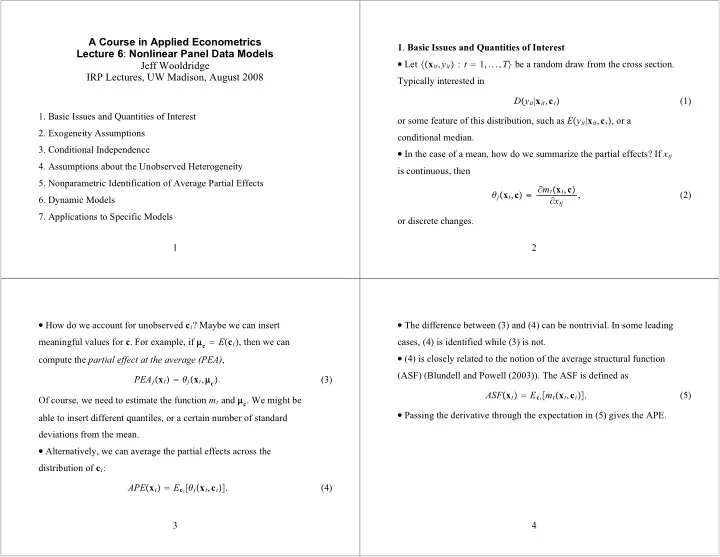
1. Basic Issues and Quantities of Interest

Let xit,yit : t 1,...,T be a random draw from the cross section.

Typically interested in Dyit|xit,ci (1)

r some feature of this distribution, such as Eyit|xit,ci, or a

conditional median.

In the case of a mean, how do we summarize the partial effects? If xtj

is continuous, then jxt,c mtxt,c xtj , (2)

r discrete changes.

2

How do we account for unobserved ci? Maybe we can insert

meaningful values for c. For example, if c Eci, then we can compute the partial effect at the average (PEA), PEAjxt jxt,c. (3) Of course, we need to estimate the function mt and c. We might be able to insert different quantiles, or a certain number of standard deviations from the mean.

Alternatively, we can average the partial effects across the

distribution of ci: APExt Ecijxt,ci. (4) 3

The difference between (3) and (4) can be nontrivial. In some leading

cases, (4) is identified while (3) is not.

(4) is closely related to the notion of the average structural function

(ASF) (Blundell and Powell (2003)). The ASF is defined as ASFxt Ecimtxt,ci. (5)

Passing the derivative through the expectation in (5) gives the APE.

4

SLIDE 2

How do APEs relate to parameters? Suppose

mtxt,c Gxt c, (6) where, say, G is strictly increasing and continuously differentiable. Then jxt,c jgxt c, (7) where g is the derivative of G. Then estimating j means we can sign of the partial effect, and the relative effects of any two continuous

variables. Even if G is specified, the magnitude of effects cannot be

estimated without making assumptions about the distribution of ci. 5

Altonji and Matzkin (2005) define the local average response (LAR)

as opposed to the APE or PAE. The LAR at xt for a continuous variable xtj is LARjxt mtxt,c xtj dHtc|xt, (8) where Htc|xt denotes the cdf of Dci|xit xt. “Local” because it averages out the heterogeneity for the slice of the population described by the vector xt. The APE is a “global average response.”

Definitions of partial effects do not depend on whether xt is

correlated with c. Of course, whether and how we estimate them certainly does. 6

2. Exogeneity Assumptions

As in linear case, cannot get by with just specifying a model for

Dyit|xit,ci.

The most useful definition of strict exogeneity for nonlinear panel

data models is Dyit|xi1,...,xiT,ci Dyit|xit,ci. (9) Chamberlain (1984) labeled (9) strict exogeneity conditional on the unobserved effects ci. Conditional mean version: Eyit|xi1,...,xiT,ci Eyit|xit,ci. (10) 7

The sequential exogeneity assumption is

Dyit|xi1,...,xit,ci Dyit|xit,ci. (11) Unfortunately, it is much more difficult to allow sequential exogeneity in in nonlinear models.

Neither (9) nor (10) allows for contemporaneous endogeneity of one

r more elements of xit, where, say, xitj is correlated with unobserved,

time-varying unobservables that affect yit. (Later in control function estimation.) 8

SLIDE 3

3. Conditional Independence

In linear models, serial dependence of idiosyncratic shocks is easily

dealt with, either by robust inference or GLS extensions of FE and FD. With strictly exogenous covariates, never results in biased estimation, even if it is ignored or improperly model. The situation is different with nonlinear models estimated by MLE.

The conditional independence assumption is

Dyi1,...,yiT|xi,ci

t1 T

Dyit|xit,ci (12) (where we also impose strict exogeneity). 9

In a parametric context, the CI assumption therefore reduces our task

to specifying a model for Dyit|xit,ci, and then determining how to treat the unobserved heterogeneity, ci.

In random effects and correlated random effects frameworks, CI plays

a critical role in being able to estimate the “structural” parameters and the parameters in distribution the of ci (and therefore, PAEs). In a broad class of models, CI plays no role in estimating APEs. 10

4. Assumptions about the Unobserved Heterogeneity

Random Effects Dci|xi1,...,xiT Dci. (13) Under (13), the APEs are nonparametrically identified from rtxt Eyit|xit xt. (14)

In some leading cases (RE probit and RE Tobit), if we want PEs for

different values of c, we must assume more: strict exogeneity, conditional independence, and (13) with a parametric distribution for Dci. 11 Correlated Random Effects A CRE framework allows dependence between ci and xi, but restricted in some way. In a parametric setting, we specify a distribution for Dci|xi1,...,xiT, as in Chamberlain (1980,1982), and much work

since. Can allow Dci|xi1,...,xiT to depend in a “nonexchangeable”
manner. (Chamberlain’s CRE probit and Tobit models.) Distributional

assumptions that lead to simple estimation – homoskedastic normal with a linear conditional mean — are restrictive.

Possible to drop parametric assumptions with

Dci|xi Dci|x i, (15) without restricting Dci|x i. 12

SLIDE 4

As T gets larger, can allow ci to be correlated with features of the

covariates other than just the time average. Altonji and Matzkin (2005) allow for x i in equation (15) to be replaced by other functions of xit : t 1,...,T, such as sample variances and covariance. Non-exchangeable functions, such as unit-specific trends, can be used,

too. Generally, assume

Dci|xi Dci|wi. (16) Practically, we need to specify wi and then establish that there is enough variation in xit : t 1,...,T separate from wi. 13 Fixed Effects The label “fixed effects” is used in different ways by different

researchers. One view: ci, i 1,...,N are parameters to be estimated.

Usually leads to an “incidental parameters problem” (which attentuates with large T.

A second meaning of “fixed effects” is that Dci|xi is unrestricted

and we look for objective functions that do not depend on ci but still identify the population parameters. Leads to “conditional maximum likelihood” if we can find a “sufficient statistic” such that Dyi1,...,yit|xi,ci,si Dyi1,...,yit|xi,si. (17)

The CI assumption is usually maintained.

14

5. Nonparametric Identification of Average Partial Effects

Identification of PAEs can fail even under a strong set of parametric

assumptions. In the probit model

Py 1|x,c x c, (18) the PE for a continuous variable xj is jx c. The PAE at c Ec 0 is jx. Suppose c|x ~Normal0,c

2. Then

Py 1|x x/1 c

21/2,

(19) so only the scaled parameter vector c /1 c

21/2 is identified;

and jxare not identified.

The APE is identified from Py 1|x, and is given by cjxc.

15

Panel data example due to Hahn (2001): xit is a binary indicator and

Pyit 1|xi,ci xit ci,t 1,2. (20) is not known to be identified in this model, even under conditional independence and the random effects assumption Dci|xi Dci. But the APE is E ci Eci and is identified by a difference of means for the treated and untreated groups, for either time period.

As shown in Wooldridge (2005a), identification of the APE holds if

we replace with an unknown function G and allow Dci|xi Dci|x i. 16

SLIDE 5

We can establish identification of APEs in panel data applications

very under strict exogeneity along with Dci|xi Dci|x

i. These two

assumptions identify the APEs. Write the average structural function at time t as ASFtxt Ecimtxt,ci Ex

iEmtxt,ci|x

i Ex

irtxt,x

i, (21) Given a consistent estimator of r t,, the ASF can be estimated as ASFtxt N1

i1 N

r txt,x i. (22) 17

Equation (21) holds without strict exogeneity Dci|xi Dci|x

i. But

these assumptions allow us to estimate estimate rt,: Eyit|xi EEyit|xi,ci|xi Emtxit,ci|xi mtxit,cdFc|xi mtxit,cdFc|x i rtxit,x i, (23) where Fc|xi denotes the cdf of Dci|xi Because Eyit|xi depends

nly on xit,x

i, we must have Eyit|xit,x i rtxit,x i, (24) and rt, is identified with sufficient time variation in xit. 18

6. Dynamic Models

Nonlinear models with only sequentially exogenous variables are

difficult to deal with. More is known about models with lagged dependent variables and otherwise strictly exogenous variables: Dyit|zit,yi,t1,...,zi1,yi0,ci, t 1,...,T, (25) which we assume also is Dyit|zi,yi,t1,...,yi1,yi0,ci. Suppose this distribution depends only on zit,yi,t1,ci with density ftyt|zt,yt1,c;. The joint density of yi1,...,yiT given yi0,zi,ci is

ftyt|zt,yt1,c;. (26) 19

Approaches to the “initial conditions” problem: (i) Treat the ci as

parameters to estimate (incidental parameters problem). (ii) Try to estimate the parameters without specifying conditional or unconditional distributions for ci (available in some special cases). Generally, cannot estimate partial effects.). (iii) Approximate Dyi0|ci,zi and then model Dci|zi. Leads to Dyi0,yi1,...,yiT|ziand MLE conditional on zi.(iv) Model Dci|yi0,zi. Leads to Dyi1,...,yiT|yi0,zi and MLE conditional

n yi0,zi. Wooldridge (2005b) shows this can be computationally

simple for popular models.

If mtxt,c, is the mean function Eyt|xt,c, the APEs are easy to

btain.

20

SLIDE 6

7. Applications to Specific Models

Binary and Fractional Response

Unobserved effects (UE) probit model:

Pyit 1|xit,ci xit ci, t 1,...,T. (27) Assume strict exogeneity (as always, conditional on ci) and use Chamberlain-Mundlak device under conditional normality: ci x i ai,ai|xi ~Normal0,a

(28) 21

If we still assume conditional serial independence then all parameters

are identified and MLE (RE probit) can be used.

N1 i1

N x

i and c

N1 i1

N x

i

i a

2. ci is not

generally normally distributed unless x i is. But can evaluate PEs at, say, c k c.

The APEs are identified from the ASF, which is consistently

estimated as ASFxt N1

i1 N

xt

a x i

(29) where, for example,

/1 a

21/2.

22

APEs are identified without the conditional serial independence

assumption. Use the marginal probabilities to estimate scaled

coefficients: Pyit 1|xi xita a x ia. (30)

Can used pooled probit or minimum distance or “generalized

estimating equations.”

Because the Bernoulli log-likelihood is in the linear exponential

family (LEF), exactly the same methods can be applied if 0 yit 1 – that is, yit is a “fractional” response – but where the model is for the conditional mean: Eyit|xit,ci xit ci. Full MLE difficult. 23

A more radical suggestion, but in the spirit of Altonji and Matzkin

(2005), is to just use a flexible model for Eyit|xit,x idirectly, say, Eyit|xit,x i t xit x i x i x i xit x i. Just average out over x i to get APEs.

If we have a binary response, start with

Pyit 1|xit,ci xit ci, (31) and assume CI, we can estimate without restricting Dci|xi.

Because we have not restricted Dci|xi in any way, it appears that we

cannot estimate average partial effects. 24

SLIDE 7

LFP

(1) (2) (3) (4) (5) Model Linear Probit RE Probit RE Probit FE Logit

Est. Method

FE Pooled MLE Pooled MLE MLE MLE Coef. Coef. APE Coef. APE Coef. APE Coef. kids .0389 .199 .0660 .117 .0389 .317 .0403 .644 .0092 .015 .0048 .027 .0085 .062 .0104 .125 lhinc .0089 .211 .0701 .029 .0095 .078 .0099 .184 .0046 .024 .0079 .014 .0048 .041 .0055 .083 kids — — — .086 — .210 — — — — — .031 — .071 — — lhinc — — — .250 — .646 — — — — — .035 — .079 — —

25

What would CMLE logit estimate in the model

Pyit 1|xit,ci ai xitbi, (32) where Ebi?

There are methods that allow estimation, up to scale, of the

coefficients without even specifying the distribution of uit in yit 1xit ci uit 0. (33) under strict exogeneity.conditional on ci. Arellano and Honoré (2001). 26

Simple dynamic model:

Pyit 1|zit,yi,t1,ci zit yi,t1 ci. (34) A simple analysis is available if we specify ci|zi,yi0 Normal 0yi0 zi,a

(35) Then Pyit 1|zi,yi,t1,...,yi0,ai zit yi,t1 0yi0 zi ai, (36) where ai ci 0yi0 zi. 27

Because ai is independent of yi0,zi, it turns out we can use standard

random effects probit software, with explanatory variables 1,zit,yi,t1,yi0,zi in time period t. Easily get the average partial effects, too: ASFzt,yt1 N1

i1 N

zt a ayt1 a a0yi0 zi

(37) Example in notes: dynamic labor force partication. The APE estimated from this method is about .259. If we ignore the heterogeneity, APE is .837. 28

SLIDE 8

For estimating parameters, Honoré and Kyriazidou (2000) extend an

idea of Chamberlain. With four four time periods, t 0,1,2, and 3, the conditioning that removes ci requires zi2 zi3. HK show how to use a local version of this condition to consistenty estimate the parameters. The estimator is also asymptotically normal, but converges more slowly than the usual N -rate.

The condition that zi2 zi3 have a distribution with support around

zero rules out aggregate year dummies. By design, cannot estimate magnitudes of effects. 29 Count and Other Multiplicative Models

Several options are available for models with conditional means

multiplicative in the heterogeneity, say, Eyit|xit,ci ci expxit (38) where ci 0. Under strict exogeneity, Eyit|xi1,...,xiT,ci Eyit|xit,ci, (39) the “fixed effects” Poisson estimator is attractive: it does not restrict Dyit|xi,ci, Dci|xi, or serial dependence. It is the conditional MLE derived under a Poisson and CI assumptions. Fully robust, even if yit is not a count variable! Robust inference is easy. 30

Estimation under sequential exogeneity has been studied by

Chamberlain (1992). Use moment conditions such as Eyit|xit,...,xi1,ci ci expxit. (40) Under this assumption, it can be shown that Eyit yi,t1 expxit xi,t1|xit,...,xi1 0, (41) and, because these moment conditions depend only on observed data and the parameter vector , GMM can be used to estimate , and fully robust inference is straightforward.