CS440/ECE448 Spring 2019 Final Review Solutions Problem 1 Solution: - - PDF document

CS440/ECE448 Spring 2019 Final Review Solutions Problem 1 Solution: Let S = event friend drives small car L = event friend drives large car T = event friend is at work on time P(S|T) = P(T,S)/P(T) = P(T,S) / (P(T,S)+P(T,L)) P(T,S) = P(T|S)*P(S) = 0.9*3/4 = 0.675 P(T,L) = P(T|L)*P(L) = 0.6*1/4 = 0.15 P(S|T) = 0.675 / (0.675+0.15) = 0.818 Problem 2 Solution:

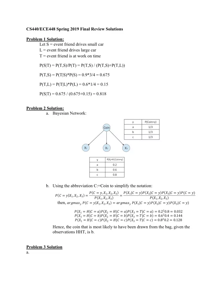
• a. Bayesian Network:
• b. Using the abbreviation C:=Coin to simplify the notation:

Hence, the coin that is most likely to have been drawn from the bag, given the

• bservations HHT, is b.

Problem 3 Solution a.

Flu Value T 3/7 F 4/7 Flu ¬Flu Sore Throat 2/3 1/2 ¬Sore Throat 1/3 1/2 Flu ¬Flu Stomach Ache 1/3 1/2 ¬Stomach Ache 2/3 1/2 Flu ¬Flu Fever 2/3 1/4 ¬Fever 1/3 3/4

• b. Let α = P(Fever, Stomach Ache, ¬Sore Throat).

P(Flu | Fever, Stomach ache, ¬Sore Throat) = (1/α) * P(Flu) * P(Stomach ache | Flu) * P(Fever | Flu) * P(¬Sore Throat | Flu) = (1/α) * 3/7 * 1/3 * 2/3 * 1/3 = (1/α) * 2/63 = (1/α) * 8 / 252. P(¬Flu | Fever, Stomach ache, ¬Sore Throat) = (1/α) * P(¬Flu) * P(Stomach ache | ¬Flu) * P(Fever | ¬Flu) * P(¬Sore Throat | ¬Flu) = (1/α) * 4/7 * 1/2 * 1/4 * 1/2 = (1/α) * 1/28 = (1/α) * (9/252). Adding these together, we have: α = (8+9)/252 = 17/ 252. Thus, the probability of having flu is 8/17. Problem 4 Solution 𝑥 ← 𝑥 + 𝜃𝑧𝑦 W1 W2 W3 Bias

• 1
• 1

1 1

• 1
• 1

1 1

• 1
• 1

1 1

• 1
• 1

1 1 2

• 1
• 1
• 1

1 Problem 5 Solution: P(X | Y=0) = ∏ 𝑄

*++ ,-*

(xi|Y=0) = a50(1-a)50 P(X | Y=1) = ∏ 𝑄

*++ ,-*

(xi|Y=1) = b50(1-b)50 P(Y=1|X) = P(X|Y=1)P(Y=1) / [P(X|Y=0)P(Y=0) + P(X|Y=1)P(Y=1)] = b50(1-b)50/[ a50(1-a)50+ b50(1-b)50] Problem 6 Solution:

• a. Yes, there are no (undirected) cycles.
• b. D and E are not independent because P(D,E) != P(D)P€. However, they are

independent given B, because P(D,E|B)=P(D|B)P(E|B).

• c. There are 6 random variables, so 26 − 1 = 63 parameters
• d. There are still 6 random variables, but each variable has 3 separate values it can take.

Thus, 36 − 1 = 728. As for conditional probability tables, we have tables for P(A), P(B|A), P(C|A), P(D|B), P(E|B), and P(F|C). The number of values for these tables are 3-1=2, 32-3=6, 32-3=6, 32-3=6, 32-3=6, 32-3=6. Adding these up, we have 2+6+6+6+6+6=32.

• e. Write down the expression for the joint probability distribution of all the variables in

the network. P(A,B,C,D,E,F)=P(A)·P(B|A)·P(C|A)·P(D|B)·P(E|B)·P(F |C)

• f. P (A = 0, B = 1, C = 1, D = 0) = P (A = 0) · P (B = 1 | A = 0) · P (C = 1 | A = 0) · P

(D = 0 | B = 1) = (1−0.8)·0.2·0.6·(1−0.5) = (1/5)(1/5)(3/5)(1/2) = 3/250

• g. P(B|A,¬D) = P(B,A,¬D)/(P(B,A,¬D)+ P(¬B,A,¬D))

P(B,A,¬D) = P(A) P(B|A)P(¬D|B) = 0.8·0.5·0.5 = 0.2 P(¬B,A,¬D)=P(A)P(¬B|A)P(¬D|¬B) = 0.8·0.5·0.4 = 0.16 So P(B|A,¬D)=0.2/0.36 = 20/36 = 5/9

• h. P(A,B,C)=P(C|A)P(B|A)P(A)

P(B,C) = sum_A P(A,B,C) P(E,B,C) = P(E|B) P(B,C) P(E,C) = sum_B P(E,B,C) Problem 7 Solution:

• a. Bayesian Network:

Table for N: depends on the prior probabilities of observing different numbers of stars. Tables for F1 and F2: F Values True f False 1-f Table for M1 (resp. M2) given F1 (resp. F2) is false (we assume that the probabilities of undercounting and overcounting are the same): M=0 M=1 M=2 M=3 M=4 N=1 e/2 1-e e/2 N=2 e/2 1-e e/2 N=3 e/2 1-e e/2 Table for M1 (resp. M2) given F1 (resp. F2) is true: M=0 M=1 M=2 M=3 M=4 N=1 1 N=2 1 N=3 1 b. M=0 M=1 M=2 M=3 M=4 N=1 (e/2)(1-f)+f (1-e)(1-f) (e/2)(1-f) N=2 f (e/2)(1-f) (1-e)(1-f) (e/2)(1-f) N=3 f (e/2)(1-f) (1-e)(1-f) (e/2)(1-f)

Problem 8 Solution:

• a. Since reward depends only on the current state, we need to have two separate

state variables for each current count: one representing a player who has decided to stop, one representing a player who has not yet decided to stop. The states are therefore: 0, 0s, 2, 2s, 3, 3s, 4, 4s, 5, 5s, 6, where the state of “6” applies to any score of 6 or more regardless of whether the player wishes to stop or draw. The actions are {Draw, Stop}.

• b. The transition function is:

𝑄(𝑂𝑡|𝑂, 𝑇𝑢𝑝𝑞) = 1 𝑄(𝑂;|𝑂, 𝐸𝑠𝑏𝑥) = ⎩ ⎪ ⎪ ⎨ ⎪ ⎪ ⎧ 1 3 𝑗𝑔 𝑂; − 𝑂 ∈ {2,3,4} 1 3 𝑗𝑔 𝑂 = 2 𝑏𝑜𝑒 𝑂; = 6 2 3 𝑗𝑔 𝑂 = 3 𝑏𝑜𝑒 𝑂; = 6 1 𝑗𝑔 𝑂 ∈ {4,5} 𝑏𝑜𝑒 𝑂; = 6 0 𝑝𝑢ℎ𝑓𝑠𝑥𝑗𝑡𝑓 The reward function is: 𝑆(𝑂𝑡) = 𝑂 𝑆(𝑂) = 0

• c. In general, for finding the optimal policy for an MDP, we would use some method

like value iteration followed by policy extraction. However, in this particular case, it is simple to work out that the optimal policy would be 𝐸𝑠𝑏𝑥 𝑗𝑔 𝑡 ≤ 2, 𝑇𝑢𝑝𝑞 𝑝𝑢ℎ𝑓𝑠𝑥𝑗𝑡𝑓 For completeness, we give below the value iteration steps based on the states and transition functions described above. The table shows only the states where the player has not yet decided to stop; from any such state, the value iteration considers two possible actions: stop, or draw. The optimal policy is given by taking the 𝑏𝑠𝑕𝑛𝑏𝑦 instead of 𝑛𝑏𝑦, in the final iteration of value iteration. V 2 3 4 5 6

V1 V2 2 3 4 5 V3 3 3 3 4 5 V4 10/3 3 3 4 5

• d. The smallest number of rounds: 4. After the first round of value iteration, the

“stop” states have learned their value, but any non-stop state still has a value of

• zero. After the fourth round, the value has converged to its correct value.

Problem 9 Solution: Unsupervised learning. When the objective is to learn the structure or the property of a given dataset. Problem 10 Solution: In this case the input space of all possible examples with their target outputs is: 1 2 2 1 1 1 1 1 1 Since there is clearly no line that can separate the two classes, this function can not be learned by a linear classifier. Problem 11 Solution:

• a. The first row of the table is correctly classified, therefore the weights are not changed.

The second row is incorrectly classified, therefore the weights are updated as W=W+(Y- Y’)F=[1,6,4]. Using these weights results in misclassification of the third row, therefore the weights are updated again to [-1,-2,-6]. Using these weights results in misclassification of the fourth row, therefore the weights are updated again to [1,4,2]. These weights correctly classify the fifth row.

• b. Yes, a perceptron can learn this function. Any weights such that w1=w2 and w0 = -8 w1

are correct; for example, the weights [-8,1,1].

• c. This problem is the arithmetic complement of the XOR problem, therefore it is not

linearly separable, and cannot be learned by a perceptron. Problem 12 Solution: convolutional layers have a lot fewer parameters than fully connected

• layers. Convolutional neurons have limited receptive fields (i.e., they respect image locality) and

their responses are shift-invariant (i.e., the same pattern will produce the same response regardless of image location). Convolution is a very traditional image feature extraction operator and is easy to implement efficiently. Problem 13 Solution: might include two of the following possibilities

• 1. Discretize the state space.
• 2. Design a lower-dimensional set of discrete features to represent the states.
• 3. Use a parametric approximator (e.g., a neural network) to estimate the Q function values

and learn the parameters instead of directly learning the state-action value functions. Problem 14: Solution TD learning computes, in each iteration, Q(s,a)=Q(s,a)+alpha(R(s)+max_{a’} Q(s’,a’)-Q(s,a)). This is an O{MN} table, whose update requires one addition per time step, so the space complexity is O{MN}. SARSA learning first chooses the action a’, then computes Q(s,a)=Q(s,a)+alpha(R(s)+Q(s’,a’)- Q(s,a)). This has the same space complexity of O{MN}. Problem 15: Solution The actor computes P(a|s), the probability that a particular action, a, is the best action to take from state s. The critic computes Q(s,a), the expected long-term discounted reward achieved by taking action a from state s. If we multiply P(a|s)Q(s,a), and add over all possible actions, we get an estimate of the value of state s. Problem 16: Solution During the time that she lived in the White House, Malia Obama owned a dog named Bo. The front door of the White House had a dog door, so that Bo could come and go as he pleased. Every Sunday, a Secret Service agent made sure that the dog door was locked. Each weekday,

• n her way to school, Malia checked the dog door. If it was locked, she unlocked it with

probability 1/3. If it was unlocked, she locked it with probability 1/4. On days when the dog door was unlocked, Bo escaped the house with probability 3/4, and went wandering about unleashed on the White House lawn. On days when the dog door was locked, the only way for Bo to escape was by begging to go out for a walk, and then breaking his leash; this happened with probability 1/10.

• a. What was the probability that Bo was found unleashed on the White House lawn on any

given Sunday? Solution: P(escape|Sunday)=1/10.

• b. Given that Bo escaped on a Monday, what was the probability that the dog door was open
• n that day?

Solution: P(escape, door open)=(1/3)(3/4)=1/4 P(escape, door closed)=(2/3)(1/10)=1/15 P(door open|escape) = (1/4)/(1/4+1/15)=15/19.

• c. A new janitor was hired at the White House. He sometimes locked the dog door, and

sometimes unlocked it. He also sometimes let Bo escape by accident; at other times, he captured Bo and brought him back inside. As a result of these changes, Malia discovered that her old model of Bo’s behavior was out of date, and had to be re-estimated. She

• bserved the following data:

Day Dog Door Bo Sunday Locked Outside Monday Unlocked Inside Tuesday Unlocked Outside Wednesday Locked Inside Thursday Locked Inside Friday Unlocked Outside Saturday Locked Inside Define Lt=1 to be the event “dog door locked on day t,” and define Ot=1 to be the event “Bo outside on day t.” Estimate the conditional probability tables P(Lt+1|Lt) and P(Ot|Lt) from the table above. Solution: P(Lt+1=1|Lt=0)=2/3 P(Lt+1=1|Lt=1)=1/3 P(Ot=1|Lt=0)=2/3 P(Ot=1|Lt=1)=1/4 Problem 17 Solution The j’th softmax output, 𝐵X, is computed from the j’th softmax input, 𝑎

X, in two steps: (1) first, 𝑎 X

is exponentiated, (2) second, exp(𝑎

X) is divided by the summation of exp(𝑎]) over all possible

values of k. Each of these two steps is necessary so that the output, 𝐵X, will satisfy all of the axioms of probability.

• a. Which of the three axioms of probability does 𝐵X satisfy only because it is proportional to

exp(𝑎

X)? State the axiom, in words, or give an equation.

Solution: The first axiom: A probability must be non-negative, i.e., 𝐵X ≥ 0.

• b. Which of the three axioms of probability does 𝐵X satisfy only because it is proportional to

1/ ∑ exp(𝑎])

𝑙

? State the axiom, in words, or give an equation. Solution: The second axiom : P(True)=1, and the third axiom : 𝑄(𝐵 ∨ 𝐶) = 𝑄(𝐵) + 𝑄(𝐶) − 𝑄(𝐵 ∧ 𝐶). Partial credit for saying that 1 = ∑ 𝐵]

]

, since that is true, but it is not an axiom of probability. Problem 18 The softmax function is given by 𝐵X =

exp 𝑎

X

∑ exp 𝑎]

]

Find 𝑒 ln 𝐵g /𝑒𝑎h. Solution : 𝑒 ln 𝐵g 𝑒𝑎h = 1 𝐵g 𝑒𝐵g 𝑒𝑎h = − 1 𝐵g

exp 𝑎g

(∑ exp 𝑎]

]

)h 𝑒 exp 𝑎h 𝑒𝑎h = −

exp 𝑎h

∑ exp 𝑎]

]

= −𝐵h Problem 19 In an HMM-DNN hybrid, the DNN softmax outputs compute 𝑄(𝑅j|𝐹j), where 𝑅j is the HMM state variable, and 𝐹j is the observed evidence at time t. Before using this probability in the HMM, we first need to divide it by 𝑄(𝑅j). Why? Solution : An HMM needs the likelihood of each state 𝑄(𝐹j|𝑅j), not the state posterior 𝑄(𝑅j|𝐹j). These two quantities are related as: 𝑄(𝐹j|𝑅j) = 𝑄(𝑅j|𝐹j)𝑄(𝐹j) 𝑄(𝑅j)

So if we compute 𝑄(𝑅j|𝐹j)/𝑄(𝑅j), that is proportional to 𝑄(𝐹j|𝑅j). The constant of proportionality is 𝑄(𝐹j), which doesn’t depend on the state variable, so it is irrelevant if our goal is to find the most probable state variable sequence (e.g., for a filtering operation, or a prediction

• peration).