CS 331: Artificial Intelligence in the last column tails black 3 - - PDF document

1

1

CS 331: Artificial Intelligence Fundamentals of Probability II

Thanks to Andrew Moore for some course material

2

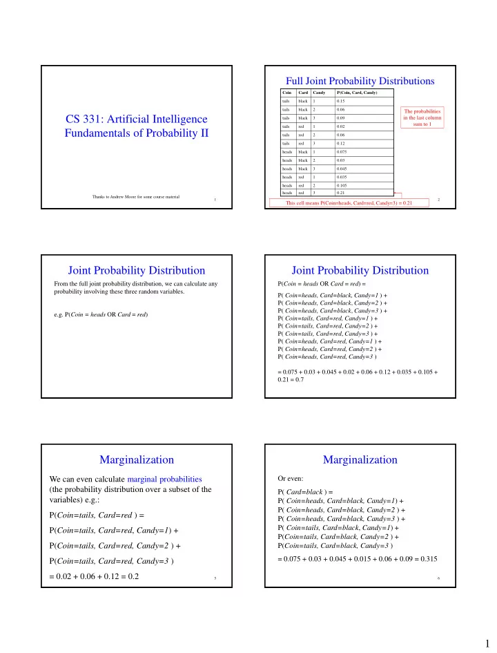
Full Joint Probability Distributions

Coin Card Candy P(Coin, Card, Candy) tails black 1 0.15 tails black 2 0.06 tails black 3 0.09 tails red 1 0.02 tails red 2 0.06 tails red 3 0.12 heads black 1 0.075 heads black 2 0.03 heads black 3 0.045 heads red 1 0.035 heads red 2 0.105 heads red 3 0.21

This cell means P(Coin=heads, Card=red, Candy=3) = 0.21 The probabilities in the last column sum to 1

Joint Probability Distribution

From the full joint probability distribution, we can calculate any probability involving these three random variables. e.g. P(Coin = heads OR Card = red)

Joint Probability Distribution

P(Coin = heads OR Card = red) = P( Coin=heads, Card=black, Candy=1 ) + P( Coin=heads, Card=black, Candy=2 ) + P( Coin=heads, Card=black, Candy=3 ) + P( Coin=tails, Card=red, Candy=1 ) + P( Coin=tails, Card=red, Candy=2 ) + P( Coin=tails, Card=red, Candy=3 ) + P( Coin=heads, Card=red, Candy=1 ) + P( Coin=heads, Card=red, Candy=2 ) + P( Coin=heads, Card=red, Candy=3 ) = 0.075 + 0.03 + 0.045 + 0.02 + 0.06 + 0.12 + 0.035 + 0.105 + 0.21 = 0.7

5

Marginalization

We can even calculate marginal probabilities (the probability distribution over a subset of the variables) e.g.: P(Coin=tails, Card=red ) = P(Coin=tails, Card=red, Candy=1) + P(Coin=tails, Card=red, Candy=2 ) + P(Coin=tails, Card=red, Candy=3 ) = 0.02 + 0.06 + 0.12 = 0.2

6

Marginalization

Or even: P( Card=black ) = P( Coin=heads, Card=black, Candy=1) + P( Coin=heads, Card=black, Candy=2 ) + P( Coin=heads, Card=black, Candy=3 ) + P( Coin=tails, Card=black, Candy=1) + P(Coin=tails, Card=black, Candy=2 ) + P(Coin=tails, Card=black, Candy=3 ) = 0.075 + 0.03 + 0.045 + 0.015 + 0.06 + 0.09 = 0.315

2

7

Marginalization

The general marginalization rule for any sets

• f variables Y and Z:





z

z) , ( ) ( Y P Y P





z

z z ) ( ) | ( ) ( P Y P Y P

• r

z is over all possible combinations of values of Z (remember Z is a set)

8

Marginalization

For continuous variables, marginalization involves taking the integral:



 z z d ) , ( ) ( Y P Y P

CW: Practice

9

Coin Card Candy P(Coin, Card, Candy) tails black 1 0.15 tails black 2 0.06 tails black 3 0.09 tails red 1 0.02 tails red 2 0.06 tails red 3 0.12 heads black 1 0.075 heads black 2 0.03 heads black 3 0.045 heads red 1 0.035 heads red 2 0.105 heads red 3 0.21

Conditional Probabilities Conditional Probabilities Conditional Probabilities

Note that 1/P(Card=black) remains constant in the two equations.

3

13

Normalization CW: Practice

14

Coin Card Candy P(Coin, Card, Candy) tails black 1 0.15 tails black 2 0.06 tails black 3 0.09 tails red 1 0.02 tails red 2 0.06 tails red 3 0.12 heads black 1 0.075 heads black 2 0.03 heads black 3 0.045 heads red 1 0.035 heads red 2 0.105 heads red 3 0.21

15

Inference

• Suppose you get a query such as

P(Card = red | Coin = heads)

Card is called the query variable (we’ll assume it’s a single variable for now) Coin is called the evidence variable because we observe it. More generally, it’s a set of variables. There are also unobserved (aka hidden) variables like Candy

16

Inference

• We will write the query as P(X | e)

This is a probability distribution hence the boldface X = Query variable (a single variable for now) E = Set of evidence variables e = the set of observed values for the evidence variables Y = Unobserved variables

Inference

We will write the query as P(X | e)



 

y

y e P e P e P ) , , ( ) , ( ) | ( X X X  

X = Query variable (a single variable for now) E = Set of evidence variables e = the set of observed values for the evidence variables Y = Unobserved variables Summation is over all possible combinations of values of the unobserved variables Y

18

Inference



 

y

y e P e P e P ) , , ( ) , ( ) | ( X X X  

Computing P(X | e) involves going through all possible entries of the full joint probability distribution and adding up probabilities with X=xi, E=e, and Y=y Suppose you have a domain with n Boolean

• variables. What is the space and time complexity of

computing P(X | e)?

4

19

Independence

• How do you avoid the exponential space

and time complexity of inference?

• Use independence (aka factoring)

20

Independence

We say that variables X and Y are independent if any of the following hold: (note that they are all equivalent)

) ( ) | ( X Y X P P  ) ( ) | ( Y X Y P P  ) ( ) ( ) , ( Y X Y X P P P 

• r
• r

21

Independence

22

Independence

23

Why is independence useful?

This table has 2 values This table has 3 values

• You now need to store 5 values to calculate P(Coin, Card,

Candy)

• Without independence, we needed 6

24

Independence

Another example:

• Suppose you have n coin flips and you want to

calculate the joint distribution P(C1, …, Cn)

• If the coin flips are not independent, you need 2n

values in the table

• If the coin flips are independent, then







n i i n

C P C C P

1 1

) ( ) ,..., (

Each P(Ci) table has 2 entries and there are n of them for a total of 2n values

5

25

Independence

• Independence is powerful!
• It required extra domain knowledge. A

different kind of knowledge than numerical

• probabilities. It needed an understanding of

relationships among the random variables.

CW: Practice

26

Coin Card Candy P(Coin, Card, Candy) tails black 1 0.15 tails black 2 0.06 tails black 3 0.09 tails red 1 0.02 tails red 2 0.06 tails red 3 0.12 heads black 1 0.075 heads black 2 0.03 heads black 3 0.045 heads red 1 0.035 heads red 2 0.105 heads red 3 0.21

Are Coin and Card independent in this distribution? Recall: for independent X and Y

) ( ) | ( X Y X P P  ) ( ) | ( Y X Y P P  ) ( ) ( ) , ( Y X Y X P P P 