Example Suppose there are five kinds of bags of candies: 10% are h 1 - - PDF document

Statistical learning

Chapter 20, Sections 1–3

Outline

♦ Bayesian learning ♦ Maximum a posteriori and maximum likelihood learning ♦ Bayes net learning – ML parameter learning with complete data – linear regression

Full Bayesian learning

View learning as Bayesian updating of a probability distribution

• ver the hypothesis space

H is the hypothesis variable, values h1, h2, . . ., prior P(H) jth observation dj gives the outcome of random variable Dj training data d = d1, . . . , dN Given the data so far, each hypothesis has a posterior probability: P(hi|d) = αP(d|hi)P(hi) where P(d|hi) is called the likelihood Predictions use a likelihood-weighted average over the hypotheses: P(X|d) = Σi P(X|d, hi)P(hi|d) = Σi P(X|hi)P(hi|d) No need to pick one best-guess hypothesis!

Example

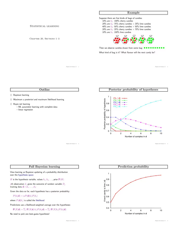
Suppose there are five kinds of bags of candies: 10% are h1: 100% cherry candies 20% are h2: 75% cherry candies + 25% lime candies 40% are h3: 50% cherry candies + 50% lime candies 20% are h4: 25% cherry candies + 75% lime candies 10% are h5: 100% lime candies Then we observe candies drawn from some bag: What kind of bag is it? What flavour will the next candy be?

Posterior probability of hypotheses

0.2 0.4 0.6 0.8 1 2 4 6 8 10 Posterior probability of hypothesis Number of samples in d P(h1 | d) P(h2 | d) P(h3 | d) P(h4 | d) P(h5 | d)

Prediction probability

0.4 0.5 0.6 0.7 0.8 0.9 1 2 4 6 8 10 P(next candy is lime | d) Number of samples in d

MAP approximation

Summing over the hypothesis space is often intractable (e.g., 18,446,744,073,709,551,616 Boolean functions of 6 attributes) Maximum a posteriori (MAP) learning: choose hMAP maximizing P(hi|d) I.e., maximize P(d|hi)P(hi) or log P(d|hi) + log P(hi) Log terms can be viewed as (negative of) bits to encode data given hypothesis + bits to encode hypothesis This is the basic idea of minimum description length (MDL) learning For deterministic hypotheses, P(d|hi) is 1 if consistent, 0 otherwise ⇒ MAP = simplest consistent hypothesis (cf. science)

ML approximation

For large data sets, prior becomes irrelevant Maximum likelihood (ML) learning: choose hML maximizing P(d|hi) I.e., simply get the best fit to the data; identical to MAP for uniform prior (which is reasonable if all hypotheses are of the same complexity) ML is the “standard” (non-Bayesian) statistical learning method

ML parameter learning in Bayes nets

Bag from a new manufacturer; fraction θ of cherry candies?

Flavor

P F=cherry ( )

θ

Any θ is possible: continuum of hypotheses hθ θ is a parameter for this simple (binomial) family of models Suppose we unwrap N candies, c cherries and ℓ = N − c limes These are i.i.d. (independent, identically distributed) observations, so P(d|hθ) =

N

• j = 1 P(dj|hθ) = θc · (1 − θ)ℓ

Maximize this w.r.t. θ—which is easier for the log-likelihood: L(d|hθ) = log P(d|hθ) =

N

• j = 1 log P(dj|hθ) = c log θ + ℓ log(1 − θ)

dL(d|hθ) dθ = c θ − ℓ 1 − θ = 0 ⇒ θ = c c + ℓ = c N Seems sensible, but causes problems with 0 counts!

Multiple parameters

Red/green wrapper depends probabilistically on flavor:

P F=cherry ( )

Flavor Wrapper

P( ) W=red | F F cherry

lime

θ

θ θ

Likelihood for, e.g., cherry candy in green wrapper: P(F = cherry, W = green|hθ,θ1,θ2) = P(F = cherry|hθ,θ1,θ2)P(W = green|F = cherry, hθ,θ1,θ2) = θ · (1 − θ1) N candies, rc red-wrapped cherry candies, etc.: P(d|hθ,θ1,θ2) = θc(1 − θ)ℓ · θrc

1 (1 − θ1)gc · θrℓ 2 (1 − θ2)gℓ

L = [c log θ + ℓ log(1 − θ)] + [rc log θ1 + gc log(1 − θ1)] + [rℓ log θ2 + gℓ log(1 − θ2)]

Multiple parameters contd.

Derivatives of L contain only the relevant parameter: ∂L ∂θ = c θ − ℓ 1 − θ = 0 ⇒ θ = c c + ℓ ∂L ∂θ1 = rc θ1 − gc 1 − θ1 = 0 ⇒ θ1 = rc rc + gc ∂L ∂θ2 = rℓ θ2 − gℓ 1 − θ2 = 0 ⇒ θ2 = rℓ rℓ + gℓ With complete data, parameters can be learned separately

Example: linear Gaussian model

0.2 0.4 0.6 0.8 1 x 0 0.20.40.60.81 y 0.5 1 1.5 2 2.5 3 3.5 4 P(y |x) 0.2 0.4 0.6 0.8 1 0.1 0.2 0.3 0.4 0.5 0.6 0.7 0.8 0.9 1 y x

Maximizing P(y|x) = 1 √ 2πσe−(y−(θ1x+θ2))2

2σ2

w.r.t. θ1, θ2 = minimizing E =

N

• j = 1(yj − (θ1xj + θ2))2

That is, minimizing the sum of squared errors gives the ML solution for a linear fit assuming Gaussian noise of fixed variance

Summary

Full Bayesian learning gives best possible predictions but is intractable MAP learning balances complexity with accuracy on training data Maximum likelihood assumes uniform prior, OK for large data sets

• 1. Choose a parameterized family of models to describe the data

requires substantial insight and sometimes new models

• 2. Write down the likelihood of the data as a function of the parameters

may require summing over hidden variables, i.e., inference

• 3. Write down the derivative of the log likelihood w.r.t. each parameter
• 4. Find the parameter values such that the derivatives are zero

may be hard/impossible; modern optimization techniques help