CS 188: Artificial Intelligence Bayes Nets Representation and - PDF document

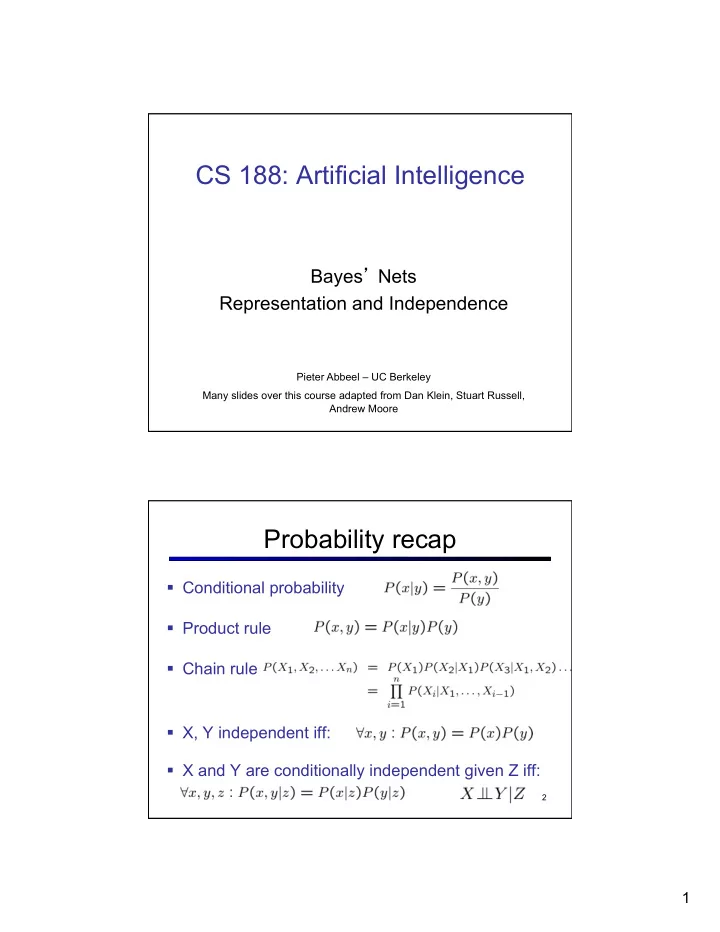
CS 188: Artificial Intelligence Bayes ’ Nets Representation and Independence Pieter Abbeel – UC Berkeley Many slides over this course adapted from Dan Klein, Stuart Russell, Andrew Moore Probability recap § Conditional probability § Product rule § Chain rule § X, Y independent iff: § X and Y are conditionally independent given Z iff: 2 1

Probabilistic Models § Models describe how (a portion of) the world works § Models are always simplifications § May not account for every variable § May not account for all interactions between variables § “ All models are wrong; but some are useful. ” – George E. P. Box § What do we do with probabilistic models? § We (or our agents) need to reason about unknown variables, given evidence § Example: explanation (diagnostic reasoning) § Example: prediction (causal reasoning) § Example: value of information 3 Bayes ’ Nets: Big Picture § Two problems with using full joint distribution tables as our probabilistic models: § Unless there are only a few variables, the joint is WAY too big to represent explicitly. For n variables with domain size d, joint table has d n entries --- exponential in n. § Hard to learn (estimate) anything empirically about more than a few variables at a time § Bayes ’ nets: a technique for describing complex joint distributions (models) using simple, local distributions (conditional probabilities) § More properly called graphical models § We describe how variables locally interact § Local interactions chain together to give global, indirect interactions 4 2

Bayes’ Nets § Representation § Informal first introduction of Bayes’ nets through causality “intuition” § More formal introduction of Bayes’ nets § Conditional Independences § Probabilistic Inference § Learning Bayes’ Nets from Data 5 Graphical Model Notation § Nodes: variables (with domains) § Can be assigned (observed) or unassigned (unobserved) § Arcs: interactions § Similar to CSP constraints § Indicate “ direct influence ” between variables § Formally: encode conditional independence (more later) § For now: imagine that arrows mean direct causation (in general, they don ’ t!) 6 3

Example: Coin Flips § N independent coin flips X 1 X 2 X n § No interactions between variables: absolute independence 7 Example: Traffic § Variables: § R: It rains R § T: There is traffic § Model 1: independence T § Model 2: rain causes traffic § Why is an agent using model 2 better? 8 4

Example: Traffic II § Let ’ s build a causal graphical model § Variables § T: Traffic § R: It rains § L: Low pressure § D: Roof drips § B: Ballgame § C: Cavity 9 Example: Alarm Network § Variables § B: Burglary § A: Alarm goes off § M: Mary calls § J: John calls § E: Earthquake! 10 5

Bayes ’ Net Semantics § Let ’ s formalize the semantics of a Bayes ’ net A 1 A n § A set of nodes, one per variable X § A directed, acyclic graph X § A conditional distribution for each node § A collection of distributions over X, one for each combination of parents ’ values § CPT: conditional probability table § Description of a noisy “ causal ” process A Bayes net = Topology (graph) + Local Conditional Probabilities 11 Probabilities in BNs § Bayes ’ nets implicitly encode joint distributions § As a product of local conditional distributions § To see what probability a BN gives to a full assignment, multiply all the relevant conditionals together: § Example: § This lets us reconstruct any entry of the full joint § Not every BN can represent every joint distribution § The topology enforces certain conditional independencies 12 6

Example: Coin Flips X 1 X 2 X n h 0.5 h 0.5 h 0.5 t 0.5 t 0.5 t 0.5 Only distributions whose variables are absolutely independent can be represented by a Bayes ’ net with no arcs. 13 Example: Traffic +r 1/4 R ¬ r 3/4 +r +t 3/4 T ¬ t 1/4 ¬ r +t 1/2 ¬ t 1/2 14 7

Example: Alarm Network E P(E) B P(B) B urglary E arthqk +e 0.002 +b 0.001 ¬ e 0.998 ¬ b 0.999 A larm B E A P(A|B,E) +b +e +a 0.95 J ohn M ary +b +e ¬ a 0.05 calls calls +b ¬ e +a 0.94 A J P(J|A) A M P(M|A) +b ¬ e ¬ a 0.06 ¬ b +e +a 0.29 +a +j 0.9 +a +m 0.7 +a ¬ j 0.1 +a ¬ m 0.3 ¬ b +e ¬ a 0.71 ¬ b ¬ e +a 0.001 ¬ a +j 0.05 ¬ a +m 0.01 ¬ b ¬ e ¬ a 0.999 ¬ a ¬ j 0.95 ¬ a ¬ m 0.99 Example Bayes ’ Net: Insurance 16 8

Example Bayes ’ Net: Car 17 Build your own Bayes nets! § http://www.aispace.org/bayes/index.shtml 18 9

Size of a Bayes ’ Net § How big is a joint distribution over N Boolean variables? 2 N § How big is an N-node net if nodes have up to k parents? O(N * 2 k+1 ) § Both give you the power to calculate § BNs: Huge space savings! § Also easier to elicit local CPTs § Also turns out to be faster to answer queries (coming) 21 Bayes’ Nets § Representation § Informal first introduction of Bayes’ nets through causality “intuition” § More formal introduction of Bayes’ nets § Conditional Independences § Probabilistic Inference § Learning Bayes’ Nets from Data 22 10

Representing Joint Probability Distributions § Table representation : d n -1 number of parameters: § Chain rule representation: number of parameters: (d-1) + d(d-1) + d 2 (d-1)+ … +d n-1 (d-1) = d n -1 Size of CPT = (number of different joint instantiations of the preceding variables) times (number of values current variable can take on minus 1) § Both can represent any distribution over the n random variables. Makes sense same number of parameters needs to be stored. § Chain rule applies to all orderings of the variables, so for a given distribution we can represent it in n! = n factorial = n(n-1)(n-2) … 2.1 23 different ways with the chain rule Chain Rule à Bayes’ net § Chain rule representation: applies to ALL distributions § Pick any ordering of variables, rename accordingly as x 1 , x 2 , … , x n Exponential in n number of parameters: (d-1) + d(d-1) + d 2 (d-1)+ … +d n-1 (d-1) = d n -1 § Bayes’ net representation: makes assumptions § Pick any ordering of variables, rename accordingly as x 1 , x 2 , … , x n § Pick any directed acyclic graph consistent with the ordering § Assume following conditional independencies: P ( x i | x 1 · · · x i − 1 ) = P ( x i | parents ( X i )) à à Joint: Linear number of parameters: (maximum number of parents = K) in n 24 Note: no causality assumption made anywhere. 11

Causality? § When Bayes ’ nets reflect the true causal patterns: § Often simpler (nodes have fewer parents) § Often easier to think about § Often easier to elicit from experts § BNs need not actually be causal § Sometimes no causal net exists over the domain § E.g. consider the variables Traffic and Drips § End up with arrows that reflect correlation, not causation § What do the arrows really mean? § Topology may happen to encode causal structure § Topology only guaranteed to encode conditional independence 25 Example: Traffic § Basic traffic net § Let ’ s multiply out the joint r 1/4 R r t 3/16 ¬ r 3/4 r ¬ t 1/16 ¬ r t 6/16 ¬ r ¬ t 6/16 r t 3/4 T ¬ t 1/4 ¬ r t 1/2 ¬ t 1/2 26 12

Example: Reverse Traffic § Reverse causality? t 9/16 T r t 3/16 ¬ t 7/16 r ¬ t 1/16 ¬ r t 6/16 ¬ r ¬ t 6/16 t r 1/3 R ¬ r 2/3 ¬ t r 1/7 ¬ r 6/7 27 Example: Coins § Extra arcs don ’ t prevent representing independence, just allow non-independence X 1 X 2 X 1 X 2 h 0.5 h 0.5 h 0.5 h | h 0.5 t 0.5 t 0.5 t 0.5 t | h 0.5 h | t 0.5 § Adding unneeded arcs isn ’ t t | t 0.5 wrong, it ’ s just inefficient 28 13

Bayes’ Nets § Representation § Informal first introduction of Bayes’ nets through causality “intuition” § More formal introduction of Bayes’ nets § Conditional Independences § Probabilistic Inference § Learning Bayes’ Nets from Data 29 Bayes Nets: Assumptions § To go from chain rule to Bayes’ net representation, we made the following assumption about the distribution: P ( x i | x 1 · · · x i − 1 ) = P ( x i | parents ( X i )) § Turns out that probability distributions that satisfy the above (“chain-rule à Bayes net”) conditional independence assumptions § often can be guaranteed to have many more conditional independences § These guaranteed additional conditional independences can be read off directly from the graph § Important for modeling: understand assumptions made 30 when choosing a Bayes net graph 14