CS 188: Artificial Intelligence Spring 2006 Lecture 19: Speech - PDF document

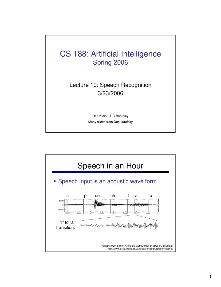
CS 188: Artificial Intelligence Spring 2006 Lecture 19: Speech Recognition 3/23/2006 Dan Klein – UC Berkeley Many slides from Dan Jurafsky Speech in an Hour � Speech input is an acoustic wave form s p ee ch l a b “l” to “a” transition: Graphs from Simon Arnfield’s web tutorial on speech, Sheffield: http://www.psyc.leeds.ac.uk/research/cogn/speech/tutorial/ 1

Spectral Analysis � Frequency gives pitch; amplitude gives volume � sampling at ~8 kHz phone, ~16 kHz mic (kHz=1000 cycles/sec) s p ee ch l a b amplitude � Fourier transform of wave displayed as a spectrogram � darkness indicates energy at each frequency y c n e u q e r f Acoustic Feature Sequence � Time slices are translated into acoustic feature vectors (~39 real numbers per slice) y c n e u q e r f …………………………………………….. a 12 a 13 a 12 a 14 a 14 ……….. � Now we have to figure out a mapping from sequences of acoustic observations to words. 2

The Speech Recognition Problem � We want to predict a sentence given an acoustic sequence: = * arg max ( | ) s P s A s � The noisy channel approach: � Build a generative model of production (encoding) = ( , ) ( ) ( | ) P A s P s P A s � To decode, we use Bayes’ rule to write = * arg max ( | ) s P s A s = arg max ( ) ( | ) / ( ) P s P A s P A s = arg max ( ) ( | ) P s P A s s � Now, we have to find a sentence maximizing this product � Why is this progress? Other Noisy-Channel Processes � Handwriting recognition ∝ ( | ) ( ) ( | ) P text strokes P text P strokes text � OCR ∝ ( | ) ( ) ( | ) P text pixels P text P pixels text � Spelling Correction ∝ ( | ) ( ) ( | ) P text typos P text P typos text � Translation? ∝ ( | ) ( ) ( | ) P english french P english P french english 3

Digitizing Speech She just had a baby � What can we learn from a wavefile? � Vowels are voiced, long, loud � Length in time = length in space in waveform picture � Voicing: regular peaks in amplitude � When stops closed: no peaks: silence. � Peaks = voicing: .46 to .58 (vowel [iy], from second .65 to .74 (vowel [ax]) and so on � Silence of stop closure (1.06 to 1.08 for first [b], or 1.26 to 1.28 for second [b]) � Fricatives like [sh] intense irregular pattern; see .33 to .46 4

Examples from Ladefoged pad bad spat Simple Periodic Sound Waves 0.99 0 –0.99 0 0.02 Time (s) � Y axis: Amplitude = amount of air pressure at that point in time � Zero is normal air pressure, negative is rarefaction � X axis: time. Frequency = number of cycles per second. � Frequency = 1/Period � 20 cycles in .02 seconds = 1000 cycles/second = 1000 Hz 5

Adding 100 Hz + 1000 Hz Waves 0.99 0 –0.9654 0 0.05 Time (s) Spectrum Frequency components (100 and 1000 Hz) on x-axis Amplitude 1000 Frequency in Hz 100 6

Part of [ae] from “had” � Note complex wave repeating nine times in figure � Plus smaller waves which repeats 4 times for every large pattern � Large wave has frequency of 250 Hz (9 times in .036 seconds) � Small wave roughly 4 times this, or roughly 1000 Hz � Two little tiny waves on top of peak of 1000 Hz waves Back to Spectra � Spectrum represents these freq components � Computed by Fourier transform, algorithm which separates out each frequency component of wave. � x-axis shows frequency, y-axis shows magnitude (in decibels, a log measure of amplitude) � Peaks at 930 Hz, 1860 Hz, and 3020 Hz. 7

Mel Freq. Cepstral Coefficients � Do FFT to get spectral information � Like the spectrogram/spectrum we saw earlier � Apply Mel scaling � Linear below 1kHz, log above, equal samples above and below 1kHz � Models human ear; more sensitivity in lower freqs � Plus Discrete Cosine Transformation Final Feature Vector � 39 (real) features per 10 ms frame: � 12 MFCC features � 12 Delta MFCC features � 12 Delta-Delta MFCC features � 1 (log) frame energy � 1 Delta (log) frame energy � 1 Delta-Delta (log frame energy) � So each frame is represented by a 39D vector � For your projects: � We’ll just use two frequencies: the first two formants 8

Why these Peaks? � Articulatory facts: � Vocal cord vibrations create harmonics � The mouth is a selective amplifier � Depending on shape of mouth, some harmonics are amplified more than others Vowel [i] sung at successively higher pitch. 2 1 3 5 6 4 7 Figures from Ratree Wayland slides from his website 9

Deriving Schwa � Reminder of basic facts about sound waves � f = c/ λ � c = speed of sound (approx 35,000 cm/sec) � A sound with λ =10 meters: f = 35 Hz (35,000/1000) � A sound with λ =2 centimeters: f = 17,500 Hz (35,000/2) Resonances of the vocal tract � The human vocal tract as an open tube Closed end Open end Length 17.5 cm. � Air in a tube of a given length will tend to vibrate at resonance frequency of tube. � Constraint: Pressure differential should be maximal at (closed) glottal end and minimal at (open) lip end. Figure from W. Barry Speech Science slides 10

From Sundberg Computing the 3 Formants of Schwa � Let the length of the tube be L � F 1 = c/ λ 1 = c/(4L) = 35,000/4*17.5 = 500Hz � F 2 = c/ λ 2 = c/(4/3L) = 3c/4L = 3*35,000/4*17.5 = 1500Hz � F 1 = c/ λ 2 = c/(4/5L) = 5c/4L = 5*35,000/4*17.5 = 2500Hz � So we expect a neutral vowel to have 3 resonances at 500, 1500, and 2500 Hz � These vowel resonances are called formants 11

From Mark Liberman’s Web site Seeing formants: the spectrogram 12

How to read spectrograms � bab : closure of lips lowers all formants: so rapid increase in all formants at beginning of "bab ” � dad : first formant increases, but F2 and F3 slight fall � gag : F2 and F3 come together: this is a characteristic of velars. Formant transitions take longer in velars than in alveolars or labials From Ladefoged “A Course in Phonetics” HMMs for Speech 13

HMMs for Continuous Observations? � Before: discrete, finite set of observations � Now: spectral feature vectors are real-valued! � Solution 1: discretization � Solution 2: continuous emissions models � Gaussians � Multivariate Gaussians � Mixtures of Multivariate Gaussians � A state is progressively: � Context independent subphone (~3 per phone) � Context dependent phone (=triphones) � State-tying of CD phone Viterbi Decoding 14

ASR Lexicon: Markov Models Viterbi with 2 Words + Unif. LM � Null transition from the end-state of each word to start-state of all (both) words. Figure from Huang et al page 612 15

Markov Process with Unigram LM Figure from Huang et al page 617 Markov Process with Bigrams Figure from Huang et al page 618 16