Correction and Preprocessing Methods Veselin Dikov 1. Beam - - PDF document

Moscow-Bavarian Joint Advanced Student School 19-29 March 2006, Moscow, Russia 1 of 5

Correction and Preprocessing Methods

Veselin Dikov

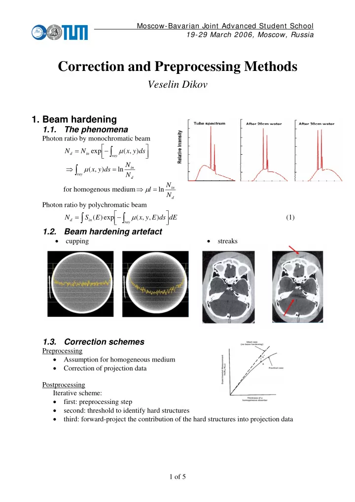
• 1. Beam hardening

1.1. The phenomena

Photon ratio by monochromatic beam ⎥ ⎦ ⎤ ⎢ ⎣ ⎡− =

∫

ray in d

ds y x N N ) , ( exp μ

d in ray

N N ds y x ln ) , ( = ⇒ ∫ μ for homogenous medium

d in

N N l ln = ⇒ μ Photon ratio by polychromatic beam

∫ ∫

⎥ ⎦ ⎤ ⎢ ⎣ ⎡− = dE ds E y x E S N

ray in d

) , , ( exp ) ( μ (1)

1.2. Beam hardening artefact

• cupping
• streaks

1.3. Correction schemes

Preprocessing

• Assumption for homogeneous medium
• Correction of projection data

Postprocessing Iterative scheme:

• first: preprocessing step
• second: threshold to identify hard structures
• third: forward-project the contribution of the hard structures into projection data

Moscow-Bavarian Joint Advanced Student School 19-29 March 2006, Moscow, Russia 2 of 5 Dual-energy Substitute ) ( ) , ( ) ( ) , ( ) , , (

2 1

E f y x a E g y x a E y x

KN

+ = μ in (1) (2)

[ ]

∫ ∫

= = + − = ⇒

ray i i KN in d

i ds y x a A dE E f A E g A E S N 2 , 1 ) , ( )) ( ) ( ( exp ) (

2 1

for , where Two scans with different voltage (different energy curves)

[ ] [ ]

∫ ∫

+ − = + − = dE E f A E g A E S A A I dE E f A E g A E S A A I

KN KN

)) ( ) ( ( exp ) ( ) , ( )) ( ) ( ( exp ) ( ) , (

2 1 2 2 1 2 2 1 1 2 1 1

Reconstruct and now ) , (

1

y x a ⇒ ) , (

2

y x a ) , , ( E y x μ can be reconstructed for any energy

• 2. Scattered radiation

Scattered radiation is a radiation that is deflected in the scanned medium.

2.1. Scatter-to-Primary Ratio (SPR)

Broad beam model estimation for SPR

( )

⎟ ⎟ ⎠ ⎞ ⎜ ⎜ ⎝ ⎛ + − + − + =

2 2 2 2 2

1 2 s R s R L R L L SPR

stβ

μ

st

μ - scattering attenuation coefficient β - fraction of scattered photons which are scattered forward

2.2. Scatter artefacts

Loss of contrast Contrast without scatter:

b b

t C ) ( μ μ − =

• linearly depends on

material thickness Contrast with scatter: SPR e SPR C

b

+ + =

− − ) (

1 ln

μ μ

• no linear

dependence

Moscow-Bavarian Joint Advanced Student School 19-29 March 2006, Moscow, Russia 3 of 5 Loss of sharpness Transmitted radiation:

sr p t

I I I + = , where

sr p sr

h I SPR I ∗ ∗ ⋅ =

sr

h - blurring kernel due to scattered radiation ∗ ∗ - 2D convolution1 Detected radiation: ⇒ ∗ ∗ + − =

vg t t d

h I I I ρ ρ) 1 (

vg sr p p sr p p d

h h I SPR I h I SPR I I ∗ ∗ ∗ ∗ ⋅ + + ∗ ∗ ⋅ + − = ) ( ) )( 1 ( ρ ρ

vg

h - blurring kernel due to veiling glare ρ - fraction of veiling

2.3. Scatter Reduction Approaches

• Anti-scatter grid
• Air gaps
• Beam collimation

2.4. Scatter Measurement

• Opaque discs techniques
• Aperture techniques
• Hybrid techniques

2.5. Scatter Correction Schemes

Convolution filtering Filter the smooth scatter signal from the image

s p p s p d

h I SPR I I I I ∗ ∗ ⋅ + = + =

s p d p

h I SPR I I ∗ ∗ ⋅ − = ⇒ Use as an estimation for , W- ratio of scatter signal to the total signal

d

I

p

I ) (

s d d p

h I W I I ∗ ∗ − = Low-pass filtered version of the detected signal. Has to be filtered out

1 2D convolution -

∫ ∫

∞ ∞ − ∞ ∞ −

− − = ∗ ∗ dudv v y u x h v u g y x h g ) , ( ) , ( ) , )( (

Moscow-Bavarian Joint Advanced Student School 19-29 March 2006, Moscow, Russia 4 of 5 Scatter sampling schemes

• Estimate scatter in sample points
• Opaque disc arrays
• Aperture arrays
• Interpolate “scatter surface” (it is a smooth one)
• 2D least squares fitting
• Filtration with sinc and jinc
• 2D polynomial fitting
• 2D bicubic splines
• Subtract the “scatter surface” estimation from

the image

• 3. Ring artefacts

Artefacts in the reconstructed image due to defect detector units; relevant for thirds generation CT ; only postprocessing correction possible.

3.1. Correction scheme

ROI

• 1. Select Region of Interest (ROI). No data out
• f it is considered
• 2. Translate image to polar coordinates
• 3. Construct artefact pattern by doing search in

window (red window on the image in right)

• 4. Subtract the pattern from the image
• 5. Translate

image back to Cartesian coordinages Search window Artefact pattern

Moscow-Bavarian Joint Advanced Student School 19-29 March 2006, Moscow, Russia 5 of 5

• 4. References
• T.Buzug, Einfürung in die Computertomographie, Springer-Verlag (2004)
• A.Kak and M.Slaney, Principles of Computerized Tomographic Imaging, IEEE Press

(1988)

• K.P.Maher and J.F. Malone, Computerized scatter correction in diagnostic radiology,

Contemporary Physics 38, 131-148 (1997).

• J.Sijbers and A.Postnov, Reduction of ring artefacts in high resolution micro-CT

reconstructions, Physics in Medicine and Biology Vol. 49 (07/2004)

• M.Zellerhoff et al, Low contrast 3D-reconstruction from C-arm data, Medical Imaging

SPIE, 646-655 (04/2004)