Data Preprocessing Why Data Preprocessing? Chris Williams, School - PowerPoint PPT Presentation

Data Preprocessing Why Data Preprocessing? Chris Williams, School of Informatics University of Edinburgh Data in the real world is dirty. It is: Data preparation is a big issue for data mining. Cabena et al (1998) extimate that data preparation accounts for 60% of the effort in a data mining application. • incomplete, e.g. lacking attribute values • Data cleaning • Data integration and transformation • noisy, e.g. containing errors or outliers • Data reduction • inconsistent, e.g. 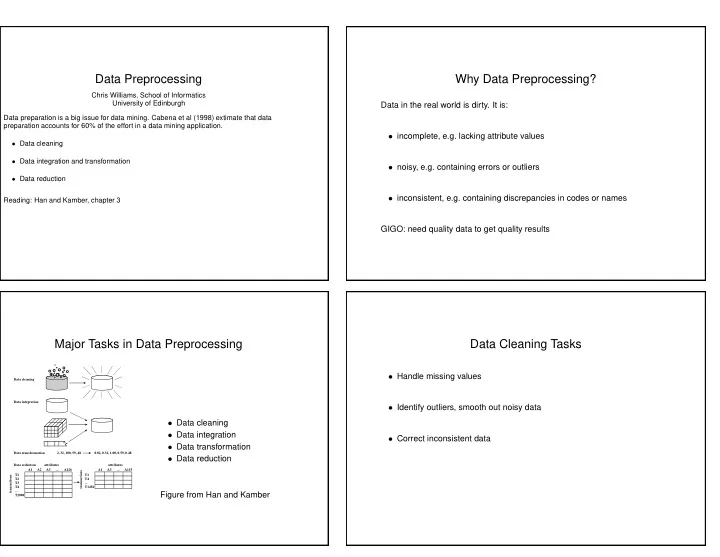containing discrepancies in codes or names Reading: Han and Kamber, chapter 3 GIGO: need quality data to get quality results Major Tasks in Data Preprocessing Data Cleaning Tasks • Handle missing values Data cleaning Data integration • Identify outliers, smooth out noisy data • Data cleaning • Data integration • Correct inconsistent data • Data transformation Data transformation 2, 32, 100, 59, 48 0.02, 0.32, 1.00, 0.59, 0.48 • Data reduction Data reduction attributes attributes A1 A2 A3 ... A126 A1 A3 ... A115 transactions T1� T1� transactions T2� T4� T3� ...� T4� T1456 ...� Figure from Han and Kamber T2000

Data Integration • Missing Data What happens if input data is missing? Is it missing at random (MAR) or is there a systematic reason for its absence? Let x m denote those values missing, and x p those Combines data from multiple sources into a coherent store values that are present. If MAR, some “solutions” are – Model P ( x m | x p ) and average (correct, but hard) • Entity identification problem: identify real-world entities from multiple data – Replace data with its mean value (?) sources, e.g. A.cust-id ≡ B.cust-num – Look for similar (close) input patterns and use them to infer missing values (crude version of density model) – Reference: Statistical Analysis with Missing Data R. J. A. Little, D. B. Rubin, Wiley • Detecting and resolving data value conflicts: for the same real-world (1987) entity, attribute values are different, e.g. measurement in different units • Outliers detected by clustering, or combined computer and human inspection Data Transformation Data Reduction • Feature selection: Select a minimum set of features ˜ x from x so that: • Normalization, e.g. to zero mean, unit standard deviation – P ( class | ˜ x ) closely approximates P ( class | x ) new data = old data − mean – The classification accuracy does not significantly decrease std deviation • Data Compression (lossy) or max-min normalization to [0 , 1] • PCA, Canonical variates new data = old data − min max − min • Sampling: choose a representative subset of the data – Simple random sampling vs stratified sampling • Normalization useful for e.g. k nearest neighbours, or for neural networks • Hierarchical reduction: e.g. country-county-town • New features constructed, e.g. with PCA or with hand-crafted features

Feature Selection Descriptive Modelling Chris Williams, School of Informatics University of Edinburgh Usually as part of supervised learning • Stepwise strategies Descriptive models are a summary of the data • (a) Forward selection: Start with no features. Add the one which is the best predictor. Then add a second one to maximize performance using first feature and new one; and • Describing data by probability distributions so on until a stopping criterion is satisfied – Parametric models • (b) Backwards elimination: Start with all features, delete the one which reduces performance least, recursively until a stopping criterion is satisfied – Mixture Models • Forward selection is unable to anticipate interactions – Non-parametric models • Backward selection can suffer from problems of overfitting – Graphical models • They are heuristics to avoid considering all subsets of size k of d features Describing data by probability distributions • Clustering – Partition-based Clustering Algorithms • Parametric models, e.g. single multivariate Gaussian – Hierarchical Clustering • Mixture models, e.g. mixture of Gaussians, mixture of Bernoullis – Probabilistic Clustering using Mixture Models • Non-parametric models, e.g. kernel density estimation Reading: HMS, chapter 9 n f ( x ) = 1 ˆ � K h ( x − x i ) n i =1 Does not provide a good summary of the data, expensive to compute on large datasets

Probability Distributions: Graphical Models Clustering Clustering is the partitioning of a data set into groups so that points in one group are similar to each other and are as different as possible from points in other groups • Mixture of Independence Models • Partition-based Clustering Algorithms C • Hierarchical Clustering X X X • Probabilistic Clustering using Mixture Models X X X 2 4 5 6 1 3 Examples (also Naive Bayes model) • Split credit card owners into groups depending on what kinds of purchases they make • Fitting a given graphical model to data • In biology, can be used to derive plant and animal taxonomies • Group documents on the web for information discovery • Search over graphical structures Defining a partition k -means algorithm • Clustering algorithm with k groups • This is a batch algo- initialize centres m 1 , . . . , m k rithm. • Mapping c from input example number to group to which it belongs while (not terminated) • There is also an on-line • In R d , assign to group j a cluster centre m j . Choose both c and the m j ’s so as to for i = 1 , . . . , n version, where the cen- minimize calculate | x i − m j | 2 for all centres tres are updated after n � | x i − m c ( i ) | 2 assign datapoint i to the closest centre each datapoint is seen i =1 end for • Also k -medoids; find • Given c , optimization of the m j ’s is easy; m j is just the mean of the data vectors recompute each m j as the mean of the a representative object assigned to class j datapoints assigned to it for each cluster centre • Optimiztion over c : cannot compute all possible groupings, use the k -means algorithm end while • Choice of k ? to find a local optimum

80 Hierarchical clustering _____________|------> p08 11 | |______|------> p04 75 7 | |------> p09 for i = 1 , . . . , n let C i = { x i } 6 |--------------------------| _______|----> p02 3 1 70 | | |--------| |----> p12 while there is more than one cluster left do | |-------------| |-------> p14 16 let C i and C j be the clusters minimizing | |________|------> p10 65 17 15 -| |------> p15 the distance D ( C i , C j ) between any two clusters 5 10 13 | ________|-----> p03 60 C i = C i ∪ C j 2 | |--------------| |-----> p06 12 | | | ________|-----> 14 remove cluster C j 55 |--------------------------| |--------| |-----> 8 end | |--------> p11 9 |______________|-------> p05 50 4 |_______|------> p13 |______|-----> p16 45 15 20 25 30 35 40 45 |-----> p17 • Results can be displayed as a dendrogram • This is agglomerative clustering; divisive techniques are also possible Distance functions for hierarchical clustering Probabilistic Clustering • Single link (nearest neighbour) • Using finite mixture models, trained with EM D sl ( C i , C j ) = min x , y { d ( x , y ) | x ∈ C i , y ∈ C j } • Can be extended to deal with outlier by using an extra, broad distribution to “mop up” outliers The distance between the two closest points, one from each cluster. Can lead to “chaining”. • Can be used to cluster non-vectorial data, e.g. mixtures of Markov models for sequences • Complete link (furthest neighbour) D cl ( C i , C j ) = max x , y { d ( x , y ) | x ∈ C i , y ∈ C j } • Methods for comparing choice of k • Disadvantage: parametric assumption for each component • Centroid measure: distance between clusters is difference between centroids • Disadvantage: complexity of EM relative to e.g. k -means • Others possible

Graphical Models: Causality Causal Bayesian Networks Season A causal Bayesian network is a • J. Pearl, Causality , Cambridge UP (2000) X Bayesian network in which each arc 1 Rain Sprinkler is interpreted as a direct causal in- • To really understand causal structure, we need to predict effect of X X fluence between a parent node and 2 3 interventions a child node, relative to the other nodes in the network. X Wet 4 (Gregory Cooper, 1999, section 4) • Semantics of do ( X = 1) in a causal belief network, as opposed to conditioning on X = 1 Slippery Causation = behaviour under inter- X 5 ventions • Example: smoking and lung cancer An Algebra of Doing Truncated factorization formula • Available: algebra of seeing (observation) ′ � � j � = i P ( x j | pa j ) if x i = x ′ i e.g. what is the chance it rained if we see that the grass is wet? P ( x 1 , . . . , x n | ˆ x i ) = ′ 0 if x i � = x i P ( rain | wet ) = P ( wet | rain ) P ( rain ) /P ( wet ) • Needed: algebra of doing  P ( x 1 ,...,x n ) ′ if x i = x  e.g. what is the chance it rained if we make the grass wet? ′ i  P ( x ′ P ( x 1 , . . . , x n | ˆ i ) = i | pa i ) x ′ 0 if x i � = x   i P ( rain | do ( wet )) = P ( rain )