Continuous Random Variables For a discrete variable X, the cumulative - PowerPoint PPT Presentation

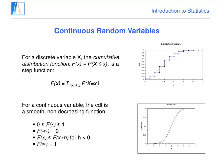
Introduction to Statistics Continuous Random Variables For a discrete variable X, the cumulative distribution function , F(x) = P(X ≤ x) , is a step function: F(x) = Σ i:xi ≤ x P(X=x i ) For a continuous variable, the cdf is a smooth, non decreasing function.  0 ≤ F(x) ≤ 1  F(- ∞) = 0  F(x) ≤ F(x+h) for h > 0  F (∞) = 1

Introduction to Statistics The density function For a discrete variable X, the probability mass function is P(X = x), which is positive at a discrete set of values x 1 , x 2 , … 0 ≤ P(X=x) ≤ 1, Σ i P(X=x i ) = 1 For a strictly continuous variable, P(X=x) = 0 ! Instead we have a density function , f(x).  0 ≤ f(x)  The area under the density up to x is the same as F(x) = P(X ≤ x).  The area under the whole density is 1.

Introduction to Statistics The normal or gaussian distribution Many variables have a bell shaped density. Examples: • Weights of a population of the same age and sex. • Heights of the same population. • The grades in a course ( urban myth ). To say that a continuous variable X, has a normal distribution with mean  and standard deviation  , we write: X ~ N(  ,  2 )

Introduction to Statistics The standard normal distribution The normal distribution with mean 0 and standard deviation 1 is called the standard normal distribution. There are tables which allow us to calculate the probabilities for this distribution, N(0,1). If we have a normal r.v., X with mean  and standard deviation  we can convert this to a standard, N(0,1) r.v. using the transformation:   X  Z 

Introduction to Statistics Examples Let Z ~ N(0,1). Calculate the following probabilities: • P(Z < -1) • P(Z > 1) • P(-1,5 < Z < 2) Calculate the 90%, 95%, 97,5% and 99% percentiles of the standard normal distribution. (These values are useful in the next chapter) Let X ~ N(2,4). Calculate the following probabilities • P(X < 0) • P(-1 < X < 1)

Introduction to Statistics

Introduction to Statistics

Introduction to Statistics Calculation with Excel It is easier to do the calculations with Excel… with the standard normal … … or directly with the original distribution.

Introduction to Statistics Approximation of the binomial distribution using a normal When n is large enough, the binomial distribution, X~ B ( n, p ) , looks like a normal distribution,    , (1 ) N np np p The approximation is usually considered to be reasonable if: np > 5 and n(1-p) > 5. EXAMPLE We throw a fair coin in the air 400 times. What is the probability of getting between 180 and 210 heads?

Introduction to Statistics The exact solution using Excel for the binomial distribution is 0,833. The estimated solution using the normal approximation is 0,819. This can be improved with a continuity correction and then the exact and approximate solutions are equal to 3 decimal places, but if we have Excel, … why should we use an approximation? We will see in the next chapter.

Introduction to Statistics Example (Test) According to the last CIS survey, the mean level of satisfaction with Mariano Rajoy is 3,09 with standard deviation 2,5. If these evaluations follow a normal distribution and a person is chosen at random, then the probability that they give Rajoy a rating of less than 3,09 is: a) 0,5. b) 0. c) 1.236 d) 1.

Introduction to Statistics Example (Test) The inflation rate follows a normal distribution with mean 1 and variance 4. Which of the following Excel formulas gives the probability that inflation will be negative?

Introduction to Statistics Example: (Exam) The following table records the ratings of the government ministers in the last CIS survey: a) Supposing that the ratings of Chacón in Spain follow a normal distribution with mean 4,55 and standard deviation 2,6, calculate the probability that a Spaniard rates her below 4,55. b) For a set of three Spanish people, what is they probability that they all rate her below 5?* c) The lowest mean rated minister is González Sinde. If her ratings are normally distributed, calculate the probability that a randomly chosen * See the next slide. Spaniard rates her exactly 5.

Introduction to Statistics

Introduction to Statistics Other continuous distributions  Uniform distribution.  The exponential and gamma distributions.  How much time between consecutive “ rare events ”  How much time between k “ rare events ”.  Distributions related to the normal: chi-squared, t, F. (see next sections)  If Z is N(0,1) then Y = Z 2 is chi-squared (with 1 degree of freedom )  If Z 1 ,…, Z k are N(0,1) then Y k = Z 1 2 + … + Z k 2 is chi-squared with k degrees of freedom.  T = Z/√ Y k is Student’s t distributed with k degrees of freedom.  F = Y j /Y k is Fisher’s F distributed with j and k degrees of freedom.