Properties of the Normal Distribution MDM4U: Mathematics of Data - PDF document

n o r m a l d i s t r i b u t i o n n o r m a l d i s t r i b u t i o n Properties of the Normal Distribution MDM4U: Mathematics of Data Management Recap For a normal distribution with µ = 17 and σ = 2, what is the likelihood that a datum has a value between 15 and 21? Since 15 is one standard deviation below the mean, and 21 is What Is the Probability That. . . ? two standard deviations above it, we can use the empirical Probabilities for Normally Distributed Data rule to determine the chance of falling in the specified range. 68 / 2 = 34% of the data fall between 15 and 17. J. Garvin 95 / 2 = 47 . 5% of the data between 17 and 21. Therefore, the likelihood of a datum having a value between 15 and 21 is 34 + 47 . 5 = 81 . 5%. J. Garvin — What Is the Probability That. . . ? Slide 1/16 Slide 2/16 n o r m a l d i s t r i b u t i o n n o r m a l d i s t r i b u t i o n Probabilities Using the Normal Distribution Probabilities Using the Normal Distribution For non-integral z -scores, tables have been created that associate a specific z -score with a probability. These tables typically measure cumulative probabilities from the left . That is, P ( x ≤ k ) for some value k . 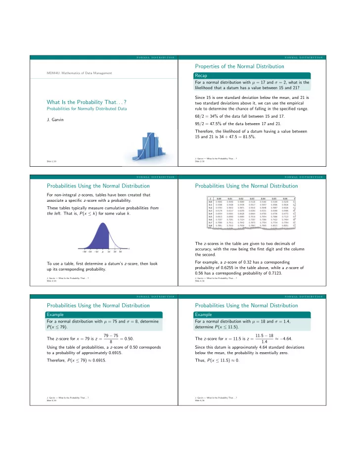The z -scores in the table are given to two decimals of accuracy, with the row being the first digit and the column the second. For example, a z -score of 0 . 32 has a corresponding To use a table, first determine a datum’s z -score, then look probability of 0 . 6255 in the table above, while a z -score of up its corresponding probability. 0 . 56 has a corresponding probability of 0 . 7123. J. Garvin — What Is the Probability That. . . ? J. Garvin — What Is the Probability That. . . ? Slide 3/16 Slide 4/16 n o r m a l d i s t r i b u t i o n n o r m a l d i s t r i b u t i o n Probabilities Using the Normal Distribution Probabilities Using the Normal Distribution Example Example For a normal distribution with µ = 75 and σ = 8, determine For a normal distribution with µ = 18 and σ = 1 . 4, P ( x ≤ 79). determine P ( x ≤ 11 . 5). The z -score for x = 79 is z = 79 − 75 The z -score for x = 11 . 5 is z = 11 . 5 − 18 = 0 . 50. ≈ − 4 . 64. 8 1 . 4 Using the table of probabilities, a z -score of 0 . 50 corresponds Since this datum is approximately 4 . 64 standard deviations to a probability of approximately 0 . 6915. below the mean, the probability is essentially zero. Therefore, P ( x ≤ 79) ≈ 0 . 6915. Thus, P ( x ≤ 11 . 5) ≈ 0. J. Garvin — What Is the Probability That. . . ? J. Garvin — What Is the Probability That. . . ? Slide 5/16 Slide 6/16

n o r m a l d i s t r i b u t i o n n o r m a l d i s t r i b u t i o n Probabilities Using the Normal Distribution Probabilities Using the Normal Distribution Most tables do not include probabilities for areas to the right Example of the curve. That is, they do not explicitly state P ( x ≥ k ) For a normal distribution with µ = 37 . 8 and σ = 2 . 4, for some k . determine P ( x ≥ 33 . 5). Recall, however, that the area under the normal curve is 1. The z -score for x = 33 . 5 is z = 33 . 5 − 37 . 8 Thus, P ( x ≥ k ) = 1 − P ( x ≤ k ). ≈ − 1 . 79. 2 . 4 The corresponding probability for a z -score of approximately − 1 . 79 is 0 . 0367. So, P ( x ≥ 33 . 5) = 1 − P ( x ≤ 33 . 5) ≈ 1 − 0 . 0367 ≈ 0 . 9633. J. Garvin — What Is the Probability That. . . ? J. Garvin — What Is the Probability That. . . ? Slide 7/16 Slide 8/16 n o r m a l d i s t r i b u t i o n n o r m a l d i s t r i b u t i o n Probabilities Using the Normal Distribution Probabilities Using the Normal Distribution Example Calculating the probability that a random variable falls between two values, a and b , is a multi-step process. For a normal distribution with µ = 93 . 8 and σ = 7 . 1, determine P ( x ≥ 67 . 9). A table will give both P ( x ≤ a ) and P ( x ≤ b ), representing the areas under the curve to a and b respectively. The z -score for x = 67 . 9 is z = 67 . 9 − 93 . 8 ≈ − 3 . 65. The area between a and b is the area to the left of b , minus 7 . 1 the area to the left of a . Since this datum is approximately 3 . 65 standard deviations below the mean, P ( x ≤ 67 . 9) ≈ 0. Therefore, P ( a ≤ x ≤ b ) = P ( x ≤ b ) − P ( x ≤ a ). Therefore, P ( x ≥ 67 . 9) = 1 − P ( x ≤ 67 . 9) ≈ 1 − 0 ≈ 1. To calculate the probability of falling between a and b , determine the z -scores for both a and b , look up their Thus, P ( x ≥ 67 . 9) ≈ 1, or essentially one. probabilities, then subtract the smaller value from the larger. J. Garvin — What Is the Probability That. . . ? J. Garvin — What Is the Probability That. . . ? Slide 9/16 Slide 10/16 n o r m a l d i s t r i b u t i o n n o r m a l d i s t r i b u t i o n Probabilities Using the Normal Distribution Probabilities Using the Normal Distribution Example Example For a normal distribution with µ = 64 and σ = 5, determine For a normal distribution with µ = 73 and σ = 5, determine P (63 ≤ x ≤ 72). P ( x = 71). The z -score for 63 is z = 63 − 64 To determine the probability of the random variable being = − 0 . 20, and for 72 is 5 exactly 71, we must use a small interval to represent the z = 72 − 64 = 1 . 60. value. But how small of an interval should be used? 5 Thus, P ( x ≤ 63) ≈ 0 . 4207, and P ( x ≤ 72) ≈ 0 . 9452. If we use the interval 70 . 9 − 71 . 1, then P ( x = 71) ≈ 0 . 0147. Therefore, P (63 ≤ x ≤ 72) ≈ 0 . 9452 − 0 . 4207 ≈ 0 . 5245. Using the interval 70 . 99 − 71 . 01, P ( x = 71) ≈ 0 . 0015. The value quickly converges toward zero. This is true for all specific probabilities P ( x = k ). J. Garvin — What Is the Probability That. . . ? J. Garvin — What Is the Probability That. . . ? Slide 11/16 Slide 12/16

n o r m a l d i s t r i b u t i o n n o r m a l d i s t r i b u t i o n Probabilities Using the Normal Distribution Reverse-Lookups Example Example The average height of a 13 year old male is 156 cm, with a What range of values corresponds to the lower 25% of all standard deviation of 4 . 2 cm. What is the probability that a data for a normal distribution with µ = 10 and σ = 1 . 5? randomly-selected 13 year old male will have a height between 150 cm and 160 cm? To answer this, we can use a reverse-lookup where we determine the z -score, based on the given probability, 0 . 25. The z -score for 150 is z = 150 − 156 ≈ − 1 . 43, and for 160 Since 0 . 25 does not appear exactly in the table, we use the 4 . 2 is z = 160 − 156 closest value, 0 . 2514, when z = − 0 . 67. ≈ 0 . 95. 4 . 2 Thus, the range will be any value less than or equal to the Thus, P ( x ≤ 150) ≈ 0 . 0764, and P ( x ≤ 160) ≈ 0 . 8289. value of the datum with a z -score of − 0 . 67. Therefore, P (150 ≤ x ≤ 160) ≈ 0 . 8289 − 0 . 0764 ≈ 0 . 7525. So, − 0 . 67 = x − 10 or x = − 0 . 67 × 1 . 5 + 10 ≈ 8 . 995. 1 . 5 The range of values is x ≤ 8 . 995. J. Garvin — What Is the Probability That. . . ? J. Garvin — What Is the Probability That. . . ? Slide 13/16 Slide 14/16 n o r m a l d i s t r i b u t i o n n o r m a l d i s t r i b u t i o n Reverse-Lookups Questions? Example What range of values corresponds to the central 10% of all data for a normal distribution with µ = 7 . 3 and σ = 0 . 4? The central 10% is the area between the lower 45% and the lower 55%. For 0 . 45, the closest z -score is 0 . 4483 for z = − 0 . 13, and for 0 . 55, the closest z -score is 0 . 5517 for z = 0 . 13. Note the symmetry. Thus, − 0 . 13 = x − 7 . 3 or x = − 0 . 13 × 0 . 4 + 7 . 3 ≈ 7 . 248. 0 . 4 Similarly, 0 . 13 = x − 7 . 3 or x = 0 . 13 × 0 . 4 + 7 . 3 ≈ 7 . 352. 0 . 4 The range of values is 7 . 248 ≤ x ≤ 7 . 352. J. Garvin — What Is the Probability That. . . ? J. Garvin — What Is the Probability That. . . ? Slide 15/16 Slide 16/16