[PDF] - CEE 370 Environmental Engineering Principles Lecture #17 PDF Document

SLIDE 1

CEE 370 Lecture #17 10/4/2019 Lecture #17 Dave Reckhow 1

David Reckhow CEE 370 L#17 1

CEE 370 Environmental Engineering Principles

Lecture #17 Ecosystems IV: Microbiology & Biochemical Pathways

Reading: Mihelcic & Zimmerman, Chapter 5

Davis & Masten, Chapter 4

Updated: 4 October 2019

Print version

David Reckhow

CEE 370 L#16

2

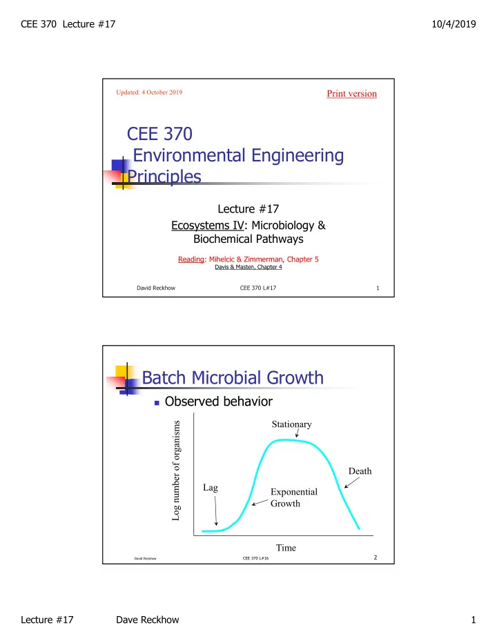
Batch Microbial Growth

 Observed behavior

Time Lag Stationary Death Exponential Growth

SLIDE 2

CEE 370 Lecture #17 10/4/2019 Lecture #17 Dave Reckhow 2

David Reckhow

CEE 370 L#16

3

Exponential Growth model

where, X = concentration of organisms at time t t = time  = proportionality constant or specific growth rate, [time─1] dX/dt =

rganism growth rate, [mass per

volume-time] N r t dN/dt

Animals

rN dt dN  X dt dX  

Bacteria

r

David Reckhow

CEE 370 L#16

4

Exp. Growth (cont.)
r

rN dt dN  rdt N dN 

rt N N



        ln

rt

e

N N 

r

X dt dX   dt X dX  

t X X



         ln

t

e

X X





Higher Organisms Microorganisms

SLIDE 3

CEE 370 Lecture #17 10/4/2019 Lecture #17 Dave Reckhow 3

David Reckhow

CEE 370 L#16

5

Exp. Growth Example

A microbial system with an ample substrate and nutrient supply has an initial cell concentration, Xo, of 500 mg/L. The specific growth rate is 0.5 /hour. a) Estimate the cell concentration after 6 hours, assuming log growth is maintained during the period. b) Determine the time required for the microbial population to double during this log growth phase.

David Reckhow

CEE 370 L#16

6

Solution I

a) To determine the microbial concentration after 6 hours, we substitute into the exp growth model,

btaining,

X = X e = 500 mg L x e

t

(0.5/hr x 6 hr) 

X = 10,000 mg L

Thus, in a period of six hours, the microorganisms increase 20 fold.

SLIDE 4

CEE 370 Lecture #17 10/4/2019 Lecture #17 Dave Reckhow 4

David Reckhow

CEE 370 L#16

7

Solution II

b) To determine the time for the concentration to double, we use the log form. Also, if the concentration doubles, then

X X = 2

r

ln X X = t



Or, solving for t we obtain,

t = ln X X = ln 2 0.5 / hr



     

t = 1.4 hr. Thus, the microbial population can double in only 1.4

hours. By comparison, the human population is currently

doubling about every 40 years.

David Reckhow

CEE 370 L#16

8

Limitations in population density

 Carrying capacity, K, and the logistic

growth model:

        K X 1

max

  X K X dt dX         1

max



                

 t t

e X X K K X

max

1



SLIDE 5

CEE 370 Lecture #17 10/4/2019 Lecture #17 Dave Reckhow 5

David Reckhow

CEE 370 L#16

9

Logistic Model (cont.)

 In many books they use different terms

when applying it to animal dynamics:

N K N r dt dN         1

 

rt

rt

t

e N K N KN e N N K K N

 

                    1

X K X dt dX         1

max



David Reckhow

CEE 370 L#16

10

Logistic Growth Example

 Determine 10 day

population for:

 Initial population:

X0 = 2 mg/L

 Max growth rate:

1 day-1

 Carrying capacity:

5000 mg/L

SLIDE 6

CEE 370 Lecture #17 10/4/2019 Lecture #17 Dave Reckhow 6

David Reckhow

CEE 370 L#16

11

Substrate-limited Growth

 Also known as resource-limited growth

 THE MONOD MODEL

where, m = maximum specific growth rate, [day-1] S = concentration of limiting substrate, [mg/L] Ks = Monod or half-velocity constant, or half saturation coefficient, [mg/L] 𝑒𝑌 𝑒𝑢

≡ 𝜈𝑌 𝜈𝑇

𝐿 𝑇 𝑌

Similar to enzyme kinetic model introduced in lecture #13

David Reckhow

CEE 370 L#16

12

Monod Kinetics

0.5*µm KS

SLIDE 7

CEE 370 Lecture #17 10/4/2019 Lecture #17 Dave Reckhow 7

Decay term

 With microorganisms, when using a substrate-limited

growth model, it is also appropriate to consider “decay”

 Decay covers the “cost of doing business”, including the

energy lost in respiration, cell maintenance & reproduction

 The mode is simple first order  And combining it with the Monod model

David Reckhow

CEE 370 L#17

13

𝑒𝑌 𝑒𝑢

𝑙𝑌

𝑒𝑌 𝑒𝑢

𝜈𝑇

𝐿 𝑇 𝑌 𝑙𝑌

Substrate model

 Yield coefficient  And  So, combining with the overall growth

model

David Reckhow

CEE 370 L#17

14

𝑍 ≡ ∆𝑌 ∆𝑇 𝑒𝑇 𝑒𝑢 1 𝑍 𝑒𝑌 𝑒𝑢 𝑒𝑇 𝑒𝑢 1 𝑍 𝑒𝑌 𝑒𝑢 1 𝑍 𝜈𝑇 𝐿 𝑇 𝑌 𝑙𝑌

SLIDE 8

CEE 370 Lecture #17 10/4/2019 Lecture #17 Dave Reckhow 8

David Reckhow

CEE 370 L#16

15

Competition for Substrate

David Reckhow

CEE 370 L#16

16

World Population Growth

SLIDE 9

CEE 370 Lecture #17 10/4/2019 Lecture #17 Dave Reckhow 9

David Reckhow

CEE 370 L#16

17

Human Population Projection

 Arithmetic Model  Exponential Model  Decreasing Rate of Increase Model  Graphical extension  Graphical comparison  Ratio method  Other

David Reckhow

CEE 370 L#16

18

Linear Model

P = Po + klt

Time kl Population

Good for some types of growth, but not all

Babies growth ~ 2 lb/month
Linear model predicts 1,320 lb by age 55

SLIDE 10

CEE 370 Lecture #17 10/4/2019 Lecture #17 Dave Reckhow 10

David Reckhow

CEE 370 L#16

19

Exponential Model

where, P = population at time t, Po = population at time zero, r (ke) = population growth rate, years-1, t = time, years.

P = P e

r t



Exponential Functions

David Reckhow

CEE 370 L#16

20

Parameter Estimation: Exponential Model

Ln P = Ln P e Ln P Ln P r t

r t

( ) ( ) ( ) ( )



  

ke or r Time (delta-t) Ln Population

SLIDE 11

CEE 370 Lecture #17 10/4/2019 Lecture #17 Dave Reckhow 11

David Reckhow

CEE 370 L#16

21

Decreasing Rate of Increase Model

P = Po + (Pmax-Po)(1-exp(-ket))

Where: Pmax is the limiting

r saturation

population

t (years)

10 20 30 40 50 60 70 80 90 100

Population

30000 35000 40000 45000 50000 55000

Decreasing Rate of Increase

Pmax= 50,000 ke = 0.04 yr-1 ke = 0.15 yr-1 ke = 0.01 yr-1

David Reckhow

CEE 370 L#16

22

Comparison of Population Models

t (years)

5 10 15 20 25 30

Population

30000 32000 34000 36000 38000 40000 42000 44000 46000 48000 50000

Decreasing Rate of Increase Linear Exponential

ke (r) = 0.014 yr-1 kl = 500 yr-1 ke = 0.04 yr-1 Pmax= 50,000

Po = 33,000 for all

SLIDE 12

CEE 370 Lecture #17 10/4/2019 Lecture #17 Dave Reckhow 12

David Reckhow

CEE 370 L#16

23

Parameter Estimation: Decreasing Rate of Increase Model Ln(Pmax-P) = Ln(Pmax-Po) - kdt

kd Ln (Pmax-P)

Time or delta-t

David Reckhow

CEE 370 L#16

24

Comparison of Population models: 100 yrs.

t (years)

10 20 30 40 50 60 70 80 90 100

Population

10000 20000 30000 40000 50000 60000 70000 80000 90000 100000 110000 120000 130000

Decreasing Rate of Increase Linear Exponential

ke = 0.04 yr-1 Pmax= 50,000 ke = 0.014 yr-1 kl = 500 yr-1

Po = 33,000 for all

SLIDE 13

CEE 370 Lecture #17 10/4/2019 Lecture #17 Dave Reckhow 13

David Reckhow

CEE 370 L#16

25

Example: World Population Growth

In 1950 the world population was estimated to be 2.5 billion. In 1990 it was estimated to be 5.5 billion. Assuming this growth rate will be sustained, a) calculate the world population in the year 2000 b) determine the year the global population will reach 10 billion.

David Reckhow

CEE 370 L#16

26

Solution

We must first calculate the population growth rate, r. To do this we convert Equation into log form:

ln P P = r t



     

SLIDE 14

CEE 370 Lecture #17 10/4/2019 Lecture #17 Dave Reckhow 14

David Reckhow

CEE 370 L#16

27

Solution, cont.

Now, if we know the population at two different times in the past, we can calculate the population growth rate, r. We know that the population in 1950 was 2.5 billion, and that it was 5.5 billion in 1990. The time change, t, is 40

years. Thus, the population growth rate is,

r = ln P Po t = ln 5.5 x 10 2.5 x 10 40 years

9 9

             r = 0.020 / yr

David Reckhow

CEE 370 L#16

28

Solution, cont.

P = P e = 5.5 x e

r

t 0.020 x (2000 - 1990) 

Population in the year 2000?

2000 in 10 x 6.7 = P

9

year

Actual: 6.1 x 109

SLIDE 15

CEE 370 Lecture #17 10/4/2019 Lecture #17 Dave Reckhow 15

David Reckhow

CEE 370 L#16

29

Solution, cont.

 t = ln P P r = ln 10 x 10 5.5 x 10 0.020 / yr

9

9

           

 t = 30years

Year that the population will reach 10 billion So 1990 + 30 is A.D. 2020

Oxygen Demand

 It is a measure of the amount of “reduced”

rganic and inorganic matter in a water

 Relates to oxygen consumption in a river or

lake as a result of a pollution discharge

 Measured in several ways

 BOD - Biochemical Oxygen Demand  COD - Chemical Oxygen Demand  ThOD - Theoretical Oxygen Demand

Dave Reckhow (UMass)

CEE 577 #12

30

SLIDE 16

CEE 370 Lecture #17 10/4/2019 Lecture #17 Dave Reckhow 16

BOD with dilution

Dave Reckhow (UMass)

CEE 577 #13

31

t i f s b

BOD = DO - DO V V       Where BODt = biochemical oxygen demand at t days, [mg/L] DOi = initial dissolved oxygen in the sample bottle, [mg/L] DOf = final dissolved oxygen in the sample bottle, [mg/L] Vb = sample bottle volume, usually 300 or 250 mL, [mL] Vs = sample volume, [mL]

When BOD>8mg/L BOD - loss of biodegradable organic matter (oxygen demand)

Dave Reckhow (UMass)

CEE 577 #13

32

Lo Lt L or BOD remaining Time Lo-Lt = BODt BOD Bottle BOD Bottle BOD Bottle BOD Bottle BOD Bottle

SLIDE 17

CEE 370 Lecture #17 10/4/2019 Lecture #17 Dave Reckhow 17

The BOD bottle curve



L=oxidizable carbonaceous material remaining to be oxidized

Dave Reckhow (UMass)

CEE 577 #13

33

5 10 15 20 25 30 35 2 4 6 8 BOD or Y (mg/L) Time (days)

BOD y L L

t t

t

  

CBOD

NBOD

Lt Lo

BOD Modeling

Dave Reckhow (UMass)

CEE 577 #13

34

"L" is modelled as a simple 1st order decay: dL

dt k L  

1

L L e

k t



 1

Which leads to: We get: BOD

y L e

t t

k t

  



( ) 1

1

BOD y L L

t t

t

  

And combining with:

SLIDE 18

CEE 370 Lecture #17 10/4/2019 Lecture #17 Dave Reckhow 18

David Reckhow

CEE 370 L#17

35

 To next lecture