
SLIDE 1
Stochastic Gradient Descent
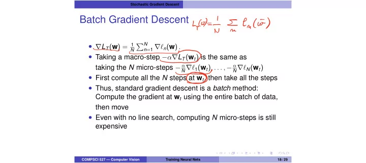
Batch Gradient Descent
- rLT(w) = 1
N
PN
n=1 r`n(w) .
- Taking a macro-step ↵rLT(wt) is the same as
taking the N micro-steps α
N r`1(wt), . . . , α N r`N(wt)
- First compute all the N steps at wt, then take all the steps
- Thus, standard gradient descent is a batch method:
Compute the gradient at wt using the entire batch of data, then move
- Even with no line search, computing N micro-steps is still
expensive
COMPSCI 527 — Computer Vision Training Neural Nets 18 / 29
Cook'T I encio