CEE 370 Environmental Engineering Principles Lecture #24 Water - PDF document

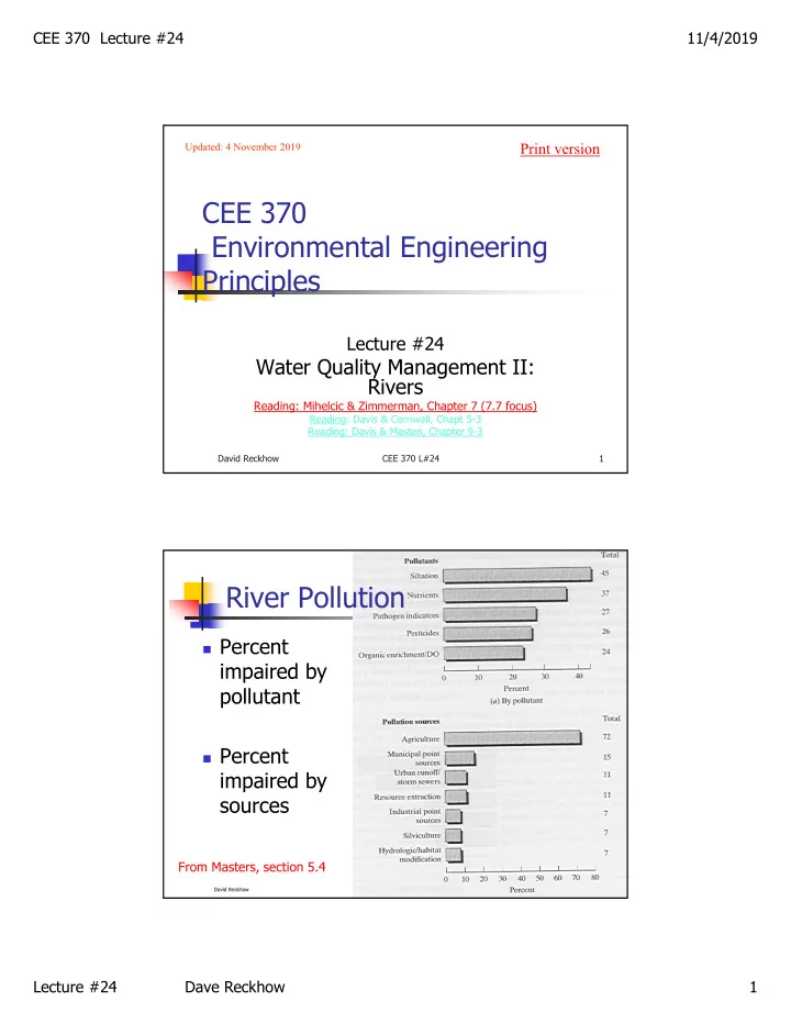
CEE 370 Lecture #24 11/4/2019 Print version Updated: 4 November 2019 CEE 370 Environmental Engineering Principles Lecture #24 Water Quality Management II: Rivers Reading: Mihelcic & Zimmerman, Chapter 7 (7.7 focus) Reading: Davis & Cornwall, Chapt 5-3 Reading: Davis & Masten, Chapter 9-3 David Reckhow CEE 370 L#24 1 River Pollution  Percent impaired by pollutant  Percent impaired by sources From Masters, section 5.4 2 CEE 370 L#24 David Reckhow Lecture #24 Dave Reckhow 1

CEE 370 Lecture #24 11/4/2019 General Aspects of WQ Models  Pollutants  Conservative  Non-conservative  Approach  Deterministic  Stochastic  Time Variability  Steady State  Dynamic 3 CEE 370 L#24 David Reckhow Waste Loading  Point Sources  Municipal WW  Industrial WW  Tributaries  Non-point Sources  Agricultural  Silvicultural  Atmospheric  Urban & Suburban Runoff 4 CEE 370 L#24 David Reckhow Lecture #24 Dave Reckhow 2

CEE 370 Lecture #24 11/4/2019 Loading Calculations Point Sources - General Concepts W(t) = Q(t)  c(t) mg/L lb/d or kg/d ft 3 /s or L/d Important Conversion Factors:      lb liters lb liters sec Kg liters sec 539 . 2 45 . 8 34 .  3    3  mg ft day mg ft day mg MG 5 CEE 370 L#24 David Reckhow Chloride Problem  Determine the required industrial reduction in chloride (a conservative substance) to maintain a desired chloride concentration of 250 mg/L at the intake Water intake Q w =6.5 MGD c w = 1500 mg/L Q=25 cfs c=30 mg/L Q T = 5 cfs c T = 30 mg/L 6 CEE 370 L#24 David Reckhow Lecture #24 Dave Reckhow 3

CEE 370 Lecture #24 11/4/2019 Example 24.1  A waste is discharged into a river  Waste characteristics  CBOD 5 = 200 mg/L  k L = 0.1 day -1     k t BOD y L ( 1 e ) 1 t t o  Q w = 1 m 3 /s  Upstream river characteristics  CBOD ultimate = 2 mg/L  Q u = 9 m 3 /s  What is the CBOD ultimate at the point of mixing? See pg. 267 in Mehelcic 7 CEE 370 L#24 David Reckhow Loading   Loading W t ( ) Qc ( ) t in  Point Sources  Municipal Wastewater Well defined origin  Industrial Wastewater easily measured more constant  Tributaries  Non-point sources  agricultural  silvicultural Diffuse origin  atmospheric more transient  urban & suburban runoff often dependent on precipitation  groundwater 8 CEE 370 L#24 David Reckhow Lecture #24 Dave Reckhow 4

CEE 370 Lecture #24 11/4/2019 Reported Values Of Selected Waste Input Parameters In The United States (Table 1.3 from Thomann & Mueller) Units a CSO c Variable Municipal Urban Agriculture Forest Atmosphere Influent b Runoff d (lb/mi 2 -d) e (lb/mi 2 -d) e (lb/mi 2 -day) f Average gcd 125 daily flow Total mg/L 300 410 610 2500 400 suspended solids g CBOD5 mg/L 180 170 27 40 8 g CBODU mg/L 220 240 g NBOD mg/L 220 290 Total mg-N/L 50 9 2.3 15 4 8.9-18.9 nitrogen Total mg-P/L 10 3 0.5 1.0 0.3 0.13-1.3 phosphorus 6 /100 Total 10 30 6 0.3 coliforms mL Cadmium  g/L 1.2 10 13 0.015 Lead  g/L 22 190 280 1.3 Chromium  g/L 42 190 22 0.088 Copper  g/L 159 460 110 Zinc  g/L 241 660 500 1.8 Total PCB  g/L 0.9 0.3 - 0.002-0.02 9 CEE 370 L#24 David Reckhow Footnotes for T&M Table 1.3 a Units apply to municipal, CSO (combined sewer overflow), and urban runoff sources; gcd = gallons per capita per day. b Thomann (1972); heavy metals and PCB, HydroQual (1982). c Thomann (1972); total coli, Tetra Tech, (1977); heavy metals Di Toro et al. (1978): PCB. Hydroscience (1978). d Tetra Tech (1977): heavy metals, Di Toro et al. (1978). e Hydroscience (1976a). f Nitrogen and phosphorus, Tetra Tech (1982): heavy metals and PC13, HydroQual (1982). g CBOD5 = 5 day carbonaceous biochemical oxygen demand (CBOD); CBODU = ultimate CBOD; NBOD = nitrogenous BOD. 10 CEE 370 L#24 David Reckhow Lecture #24 Dave Reckhow 5

CEE 370 Lecture #24 11/4/2019 Loading: Flow as a function of precipitation  Non point sources are difficult to characterize  Empirical approach: export coefficients (see Table 3.1 in T&M)  Mechanistic approach: relate to meteorology, topology, etc.  Flow: use the rational formula: Q R = cIA Drainage Area [L 2 ] Runoff flow [L 3 /T] Rainfall Intensity [L/T] Runoff coefficient 0.1-0.3 for rural areas (1 person/acre) 0.7-0.9 for heavy commercial areas Note: 1 acre-in/hr  1 cfs 11 CEE 370 L#24 David Reckhow Loading: conc. as a function of flow  It is common for pollutant concentrations from uncontrolled sources (e.g. tributaries) to be correlated with flow  establish a 1000 log-log Concentration (mg/L) relationship 100  c=aQ b 10 Log(C) = log(a) + b*log(Q) 1 1 10 100 1000 Flow (cfs) 12 CEE 370 L#24 David Reckhow Lecture #24 Dave Reckhow 6

CEE 370 Lecture #24 11/4/2019 Loading Example: #3.1 from T&M Data: Runoff from 100 mi 2 of agricultural lands drains to a point in a  river where a city of 100,000 people is located. The city has a land area of 10 mi 2 and its sanitary sewers are separated from its storm drains. A sewage treatment plant discharges to the river immediately downstream of the city. The area receives an annual rainfall of 30 in. of which 30% runs off the agricultural lands and 50% drains off the more impervious city area. Problem: Using the loading data from Table 1.3 and the residual  fractions cited in the table below, compare the contributions of the atmospheric, agricultural and urban sources to annual average values of flow, CBOD5, total coliform bacteria, and lead in the river. Neglect any decay mechanisms for all parameters. (at) (ag) (ur) Wastewater Treatment Plant Item Atmospheric Agricultural Urban Runoff Influent Resid. Fract. Fow 30% precip. 50% precip. 125 gcd 1.00 2 -d CBOD5 40 lb/mi 27 mg/L 180 mg/L 0.15 5 /100mL 6 /100mL Total coliform 100/100 mL 3x10 3x10 0.0001 2 -d Lead 1.3 lb/mi 280  g/L 22  g/L 0.05 13 CEE 370 L#24 David Reckhow Solution to loading problem  Flow contributions     2  2 5280 ft 1 ft 1 yr Q ( ag ) 100 mi 30 in / yr 0 . 3 1 d mi 12 in 365 d 86 , 400 s  66 . 3 cfs     2  2 5280 ft 1 ft 1 yr Q ( ur ) 10 mi 30 in / yr 0 . 5 1 d mi 12 in 365 d 86 , 400 s  11 . 1 cfs 125 gal  Q ( wwtp ) 100 , 000 cap 1 MG  6 cap d 10 gal    1 . 548 cfs 12 . 5 MGD MGD  19 . 4 cfs 14 CEE 370 L#24 David Reckhow Lecture #24 Dave Reckhow 7

CEE 370 Lecture #24 11/4/2019 Solution to loading problem (cont.)  CBOD5 loading   lb  W ( ag ) 100 mi 2  40  2  mi d  lb  4000 d lb / d    W ( ur ) 11 . 1 cfs 27 mg / L 5 . 4  cfs mg / L lb  1620 d      W ( wwtp ) 12 . 5 MGD 180 mg / L 0 . 15 8 . 34 lb / d MGD * mg / L lb  2810 d 15 CEE 370 L#24 David Reckhow Solution to loading problem (cont.)  Lead loading   lb  2 W ( atm ) 100 mi  1 . 3  0 . 1 2  mi d  lb  13 d    lb / d 10 3 mg       W ( ur ) 11 . 1 cfs 280 g / L 5 . 4     cfs mg / L g   lb  16 . 8 d      3   10 mg W ( wwtp ) 12 . 5 MGD 22 g / L 0 . 05 8 . 34 lb / d  MGD * mg / L g lb  0 . 11 d 16 CEE 370 L#24 David Reckhow Lecture #24 Dave Reckhow 8

CEE 370 Lecture #24 11/4/2019 DO Example A polluted stream with a temperature of 25  C has a dissolved oxygen concentration of 4 mg/L. Use Gibbs free energy to determine if oxygen from the atmosphere is dissolving into the water, the oxygen is at equilibrium, or oxygen from the stream is going into the atmosphere.  (aq) (g) O O 2 2 Example 4.7 from Ray 17 CEE 370 L#24 David Reckhow Solution to DO example = (0 kcal mol ) - (-3.9 kcal       G = G - G mol ) rxn O (g) O (aq) 2 2 = 3.9 kcal  G  rxn mol p    O G = G + RT ln 2 [O (aq)] 2 [O (aq)] = 4 mg O 1000 mg O x mol O g O 2 2 2 -4 x 32 g O = 1.25 x 10 M 2 L 2 2 18 CEE 370 L#24 David Reckhow Lecture #24 Dave Reckhow 9

CEE 370 Lecture #24 11/4/2019 Solution (cont.)  G = 3.9 kcal mol x 1000 cal  cal   0.209 atm       + 1987 . K- mol (298K) ln     kcal 1.25 x 10 M -4 cal  G = 491 mol > 0 Since  G is positive, the reaction will proceed in the reverse direction as written. From the atmosphere to the water. 19 CEE 370 L#24 David Reckhow Gas Transfer: Equilibria Henry’s Law   C K p aq H gas where, C aq = concentration of species A at equilibrium, [mol/L or mg/L] K’ H = Henry's Law constant for species A, [mol/L-atm or mg/L-atm] p gas = partial pressure gas A exerts on the liquid, [atm] 20 CEE 370 L#24 David Reckhow Lecture #24 Dave Reckhow 10