C Execution Time Analysis Jan Gustafsson, Docent Mlardalen - - PDF document

SLIDE 1

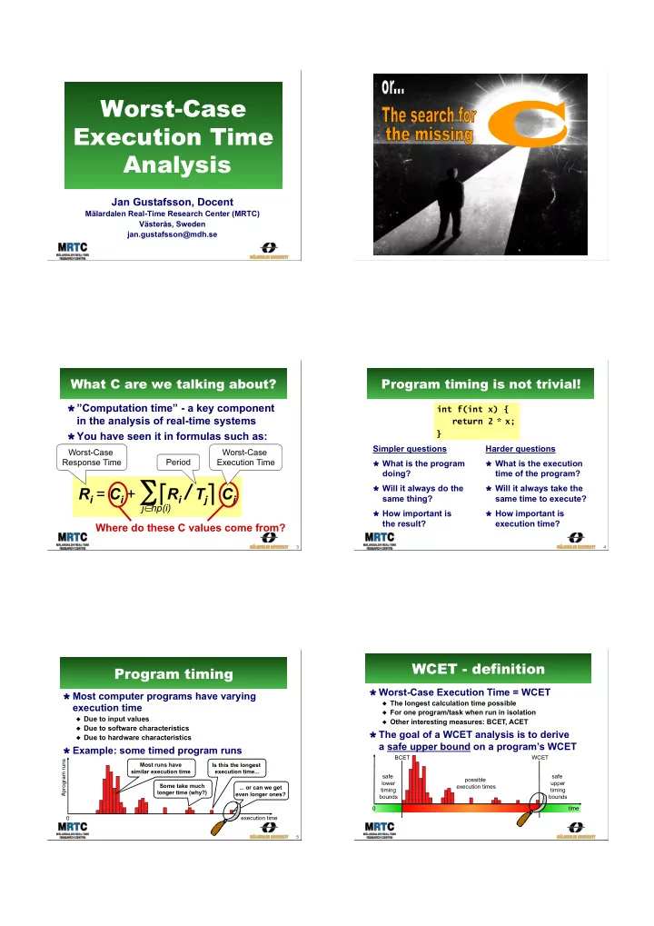
Worst-Case Execution Time Analysis

Jan Gustafsson, Docent

Mälardalen Real-Time Research Center (MRTC) Västerås, Sweden jan.gustafsson@mdh.se

2

C

3

What C are we talking about?

! ”Computation time” - a key component

in the analysis of real-time systems

! You have seen it in formulas such as:

Ri = Ci + ∑ "Ri / Tj# Cj

j∈hp(i)

Worst-Case Response Time Period

Where do these C values come from?

Worst-Case Execution Time

Program timing is not trivial!

Simpler questions

! What is the program

doing?

! Will it always do the

same thing?

! How important is

the result?

4

int f(int x) { return 2 * x; } Harder questions

! What is the execution

time of the program?

! Will it always take the

same time to execute?

! How important is

execution time?

Program timing

! Most computer programs have varying

execution time

" Due to input values " Due to software characteristics " Due to hardware characteristics

! Example: some timed program runs

5

execution time #program runs Most runs have similar execution time Some take much longer time (why?) Is this the longest execution time... ... or can we get even longer ones? safe upper timing bounds possible execution times

WCET - definition

! Worst-Case Execution Time = WCET

" The longest calculation time possible " For one program/task when run in isolation " Other interesting measures: BCET, ACET

! The goal of a WCET analysis is to derive

a safe upper bound on a program’s WCET

time safe lower timing bounds BCET WCET

SLIDE 2

Presentation outline

! Embedded system fundamentals ! WCET analysis

" Measurements " Static analysis " Flow analysis, low-level analysis, and calculation " Hybrid approaches

! WCET analysis tools ! The SWEET approach to WCET analysis ! (Multi-core + WCET analysis?) ! WCET analysis demo (SWEET)

Embedded systems fundamentals Embedded computers

! An integrated part of a larger system

" Example 1: A microwave oven contains at

least one embedded processor

" Example 2: A modern car can contain more

than 100 embedded processors ! Interacts with the user,

the environment, and with other computers

" Often limited or

no user interface

" Often with

timing constraints

input result

Embedded systems everywhere

! Today, all advanced

products contain embedded computers!

" Our society depends on

that they function correctly

11

Embedded systems software

! Amount of software can vary from

extremely small to very large

" Gives characteristics to the product

! Often developed with target

hardware in mind

" Often limited resources (memory / speed) " Often direct accesses to different HW devices " Not always easily portable to other HW

! Many different programming languages

" C still dominates, but often special purpose languages

! Many different software development tools

" Not just GCC and/or Microsoft Visual Studio

Embedded system hardware

! Huge variety of embedded

system processors

" Not just one main processor type as for PCs " Additionally, same CPU can be used with various

hardware configurations (memories, devices, …)

! The hardware is often tailored

specifically to the application

" E.g., using a DSP processor for signal

processing in a mobile telephone

! Cross-platform development

" E.g., develop on PC and download

final application to target HW

SLIDE 3 Timely Software - a Challenge 13

"Desktop" 2% "Embedded" 98%

Some interesting figures

! 4 billion embedded processors sold in 2008

" Global market worth €60 billion " Predicted annual growth rate of 14% " Forecasts predict more than 40 billion embedded devices in 2020

! Embedded processors clearly dominate yearly

production

Source: http://www.artemis-ju.eu/embedded_systems

Real-time systems

! Computer systems where the timely

behavior is a central part of the function

" Containing one or more embedded computers " Both soft- and hard real-time, or a mixture…

Timing of radio communication, speech recognition,… Timing of music playing from MP3 file Timing of radio communication, motor control, rudder and flaps control,… Timing of network communication, motor control, ABS brakes, anti-slip control,…

Uses of reliable WCET bounds

! Hard real-time systems

" WCET needed to guarantee behavior

! Real-time scheduling

" Creating and verifying schedules " Large part of RT research assume

the existence of reliable WCET bounds

! Soft real-time systems

" WCET useful for system understanding

! Program tuning

" Critical loops and paths

! Interrupt latency checking

WCET analysis

Obtaining WCET bounds

! Measurement

" Industrial practice

! Static analysis

" Research front

Measuring for the WCET

! Methodology:

" Determine ”worst-case

input” or run as many inputs as possible

" Execute and measure

the time

" Add a safety margin

18

SLIDE 4 19

Measurement issues 1

! What is the worst-case input?

" In general, the problem of determining the worst case input

value combination to an arbitrary program is very hard.

! Alternative: run all inputs?

" Typically not possible, since the number of input

combinations typically is huge.

" For example: 10 variables of size 32 bits => number of

necessary measurement runs = 4 294 967 29510

" Also keep in mind that the program state is a part of the input

! In practice: run as many inputs as possible

" There are some ideas how to test extreme cases and corners " Has the worst-case path really been taken? No guarantee!

20

Measurement issues 2

! How to measure the execution time?

" Option 1: SW methods

! Operating system clocks ! Simulators ! High-water marking

" Option 2: HW + SW methods

! Add instrumentation code ! Use oscilloscopes, logic analyzers, emulators logic analyzers or debug support ! The instrumentation may affect the timing ! Instrumentation code is often left in shipped code ! How much instrumention output can be handled? LEDs Buzzer

21

SW measurement methods

! Operating system clocks

" Commands such as time

time, date date and clock clock

" Note that all OS-based solutions require

precise HW timing facilities (and an OS)

! Cycle-level simulators

" Software simulating CPU " Correctness vs. hardware?

! High-water marking

" Keep system running " Record maximum time

• bserved for task

" Keep in shipping systems,

read at service intervals

22

Using an oscilloscope

! Common equipment for HW debugging

" Used to examine electrical output

signals of HW ! Observes the voltage or signal

waveform on a particular pin

" Usually only two to four inputs

! To measure time spent in a routine:

• 1. Set I/O pin high when entering routine
• 2. Set the same I/O pin low before exiting
• 3. Oscilloscope measures the amount of

time that the I/O pin is high

• 4. This is the time spent in the routine

23

Using a logic analyzer

! Equipment designed for

troubleshooting digital hardware

! Have dozens or even

hundreds of inputs

" Each one keeping track on

whether the electrical signal it is attached to is currently at logic level 1 or 0

" Result can be displayed

against a timeline

" Can be programmed to start

capturing data at particular input patterns

Target board HW Debugger 24

HW measurement tools

! In-circuit emulators (ICE)

" Special CPU version revealing internals ! High visibility & bandwidth ! High cost + supportive HW required

! Processors with debug support

" Designed into processor ! Use a few dedicated processor pins " Using standardized interfaces ! Nexus debug interfaces, JTAG, Embedded Trace Macrocell, … " Supportive SW & HW required " Common on modern chip

SLIDE 5

Fundamental problems when using measurements

! Measured time never exceeds WCET

How do we know that we catched the WCET?

" A safety margin must be added, but how

much is enough?

safe upper timing bounds possible execution times time safe lower timing bounds BCET WCET Only this measurement is safe (= WCET)! Measurement will result in a value ≤ WCET

Static WCET analysis

Static WCET analysis

! Do not run the program – analyze it!

" Using models based on the static properties of the

software and the hardware

! Guaranteed safe WCET bounds

" Provided all models, input data and analysis

methods are correct

! Trying to be as tight as possible

safe upper timing bounds possible execution times time safe lower timing bounds BCET WCET All derived bounds will be ≥ WCET foo(x,i): while(i < 100) if (x > 5) then x = x*2; else x = x+2; end if (x < 0) then b[i] = a[i]; end i = i+1; end

Again: Causes of Execution Time Variation

! Execution characteristics

• f the software

" A program can often execute

in many different ways

" Input data dependencies " Application characteristics

! Timing characteristics

• f the hardware

" Clock frequency " CPU characteristics " Memories used " … Analysis

WCET analysis phases

Reality

Compiler Object
 Code Target Hardware program Low level analysis Calculation Flow analysis

• 1. Flow analysis

" Bound the number of times

different program parts may be executed (mostly SW analysis)

• 2. Low-level analysis

" Bound the execution time

• f different program parts

(combined SW & HW analysis)

• 3. Calculation

" Combine flow- and low-level

analysis results to derive an upper WCET bound

Actual
 WCET WCET
 bound

30

Flow analysis

SLIDE 6 31

Flow Analysis

! Provides bounds on the number

• f times different program parts

may be executed

" Valid for all possible executions

! Examples of provided info:

" Bounds of loop iterations " Bounds on recursion depth " Infeasible paths

! Info provided by:

" Static program analysis " Manual annotations

Flow analysis Low level analysis Calculation Program WCET Estimate

The control-flow graph

foo(x,i): A: while(i < 100) B: if (x > 5) then C: x = x*2; else D: x = x+2; end E: if (x < 0) then F: b[i] = a[i]; end G: i = i+1; end

Flows as edges

foo() C A B D E F G end

Each block will run as a unit

Example program

Flow info characteristics

Basic finiteness Statically allowed Actual feasible paths

Loop bound: 100

#F < 10

Control flow graph

Structurally possible executions (infinite)

Relation between possible executions and flow info

WCET found here = desired result

foo(x,i): A: while(i < 100) B: if (x > 5) then C: x = x*2; else D: x = x+2; end E: if (x < 0) then F: b[i] = a[i]; end G: i = i+1; end foo() C B D E F G end A

WCET found here =

• verestimation

Example: Loop bounds

! Loop bound:

" Depends on possible values

• f input variable i

! E.g. if 1 ≤ i ≤ 10 holds for input value i, then loop bound is 100 " In general, a very difficult

problem

" However, solvable for many

types of loops

! Requirement for basic

finiteness (a WCET)

" All loops must be

upper bound foo(x,i): A: while(i < 100) B: if (x > 5) then C: x = x*2; else D: x = x+2; end E: if (x < 0) then F: b[i] = a[i]; end G: i = i+1; end

Example: Infeasible path

! Infeasible path:

" Path A-B-C-E-F-G

can not be executed since C implies ¬F

" If (x > 5) then it is not

possible that (x*2) < 0 ! Limits statically

allowed executions

" Might tighten the

WCET estimate

foo(x,i): A: while(i < 100) B: if (x > 5) then C: x = x*2; else D: x = x+2; end E: if (x < 0) then F: b[i] = a[i]; end G: i=i+1; end

36

Example: Triangular Loop

! Two loops:

" Loop A bound: 100 " Local B bound: 100

! Block C:

" By loop bounds:

100 * 100 = 10 000

" But actually:

100+...+1 = 5 050 ! Limits statically

allowed executions

" Might tighten the

WCET estimate

triangle(a,b): A: loop(i=1..100) B: loop(j=i..100) C: a[i,j]=... end loop end loop

SLIDE 7

int$i=0;$ ...$$ while(i<100)$ {$ $$...$$ $$i++;$ }$ ...$

The mapping problem

! Flow analysis easier on source code level

" Semantics of code clearer " Easier for programmer/tool to derive flow info

! Low-level analysis requires binary code

" The code executed by the processor

! Question: How to safely map flow source code level

flow information to binary code?

...$ 0111111010010111$ 0110010100101001$ 1001010100111010$ 1001010011111110$ 1010010101010100$ 1001010101010101$ ...$

Loop bound (header): 101 Where is the loop?

Source code Executable

The mapping problem (cont)

! Embedded compilers often do a lot of code optimizations

" Important to fit code and data into limited memory resources

! Optimizations may significantly change code (and data) layout

" After optimizations flow info may no longer be valid

! Solutions:

" Use special compiler also mapping flow info (not common) " Use compiler debug info for mapping (only works with little/no optimizations) " Perform flow analysis on binaries (most common) 38

$int$i=0;$ $...$$ $while(i<100)${$ $$$...$$ $$$i++;$ $}$ $...$ $int$i=0;$ $...$$ $do${$ $$$...$$ $$$i++;$ $}$while(i<100)$ $...$

Flow analysis: Loop condition taken 101 times Compiler: i=0 always holds at first execution

• f loop condition

Loop condition taken 100 times Before optimization After optimization

Executable

1000110000011110 1000110000100000 1010110000100000 1010110000011110 1010110000100011 1010111100011001

Linker Object File Object File Object File

twice: mov ip, sp stmfd sp!, {fp,ip,lr,pc} sub fp, ip, #4 sub sp, sp, #8 str r0, [fp, #-16] ldr r3, [fp, #-16] mov r3, r3, asl #1 str r3, [fp, #-20] ldr r3, [fp, #-20] mov r0, r3 ldmea fp, {fp,sp,pc}

Compiler

Embedded SW Tool Chain

C Source C Source C Library C Runtime Start-up OS C Source WCET

int twice(int a) { int temp; temp = 2 * a; return temp; }

Affects timing Affects timing Affects timing Affects timing Affects timing Affects timing Affects timing

40

The SW building tools

! The compiler:

" Translates an source code file to an object code file ! Only translates one source code file at the time " Often makes some type of code optimizations ! Increase execution speed, reduce memory size, … ! Different optimizations give different object code layouts

! The linker:

" Combines several object code files into one executable ! Places code, global data, stack, etc in different memory parts ! Resolves function calls and jumps between object files " Can also perform some code transformations

! Both tools may affect the program timing!

41

Example: compiling & linking

/****************** * File: main.c *****************/ int foo(); int main() { return 1 + foo(); } /****************** * File: foo.c *****************/ int foo() { return 1; } Contains object code for main.c Object code contains an unresolved call to foo

Compiler

main.o

Contains object code for foo.c

Compiler

foo.o

The main.o and foo.o object code files are combined The call to foo in main has been resolved

Linker

a.exe

42

Common additional files

! C Runtime code:

" Whatever needed but not supported by the HW ! 32-bit arithmetic on a 16-bit machine ! Floating-point arithmetic ! Complex operations (e.g., modulo, variable-length shifts) " Comes with the compiler " May have a large footprint ! Bigger for simpler machines ! Tens of bytes of data and tens of kilobytes of code

! OS code:

" In many ES the OS code is linked together with the rest

• f the object code files to form a single binary image

SLIDE 8 43

Common additional files

! Startup code:

" A small piece of assembly code that prepares the way for

the execution of software written in a high-level language

! For example, setting up the system stack

" Many ES compilers provide a file named

startup.asm, crt0.s, … holding startup code ! C Library code:

" A full ANSI-C compiler must provide code that implements

all ANSI-C functionality

! E.g., functions such as printf, memmove, strcpy

" Many ES compilers only support subset of ANSI-C " Comes with the compiler (often non-standard)

Low-level analysis

Low-Level Analysis

! Determine execution time bounds

for program parts

" Focus of most WCET-related research

! Using a model of the target HW

" The model does not need to model all

HW details

" However, it should safely account for

all possible HW timing effects ! Works on the binary, linked code

" The executable program

Flow analysis Program Low level analysis Calculation WCET Estimate

Some HW model details

! Much effort required to safely model CPU internals

" Pipelines, branch predictors, superscalar, out-of-order, …

! Much effort to safely model memories

" Cache memories must be modelled in detail " Other types of memories may also affect timing

! For complex CPUs many features must be

analyzed together

" Timing of instructions gets history dependant

! Developing a safe HW timing model troublesome

" May take many months (or even years) " All things affecting timing must be accounted for

Hardware time variability

! Simpler 4-, 8- & 16-bit processors (H8300, 8051, …):

" Instructions might have varying execution time due to

argument values

" Varying data access time due to different memory areas " Analysis rather simple, timing fetched from HW manual

! Simpler 16- & 32-bit processors, with a (scalar) pipe-

line and maybe a cache (ARM7, ARM9, V850E, …):

" Instruction timing dependent on previously

executed instructions and accessed data: ! State of pipeline and cache

" Varying access times due to cache hits and misses " Varying pipeline overlap between instructions " Hardware features can be analyzed in isolation

Hardware time variability

! Advanced 32- & 64-bit processors (PowerPC 7xx,

Pentium, UltraSPARC, ARM11, …):

" Many performance enhancing features affect timing

! Pipelines, out-of-order exec, branch pred., caches, speculative exec. ! Instruction timing gets very history dependent

" Some processors suffer from timing anomalies

! E.g., a cache miss might give shorter overall program execution time than a cache hit

" Features and their timing interact

! Most features must be analyzed together

" Hard to create a correct and safe

hardware timing model! ! Multi-cores - discussed later

SLIDE 9 49

Example: CPU pipelines

! Observation: Most instructions go through

same stages in the CPU

! Example: Classic RISC 5-stage pipeline IF ID EX MEM WB

Instruction fetch (IF) Get the next instruction from memory to process (its address is held by PC) Instruction decode Determine operation to be performed (i.e., extract

• pcode and arguments)

Execute Perform the actual

• peration (e.g, an add)

Memory access Load/store values from/to memory if needed Write back Write the result into the target register

50

CPU pipelines

! Idea: Overlap the CPU stages of the instruct-

ions to achieve speed-up

! No pipelining:

" Next instruction

cannot start before previous one has finished all its stages

! Pipelining:

" In principle: speedup = pipeline length " However, often dependencies

between instructions

IF ID EX MEM WB 1 2 3 5 6 4 IF ID EX MEM WB 1 2 3 5 6 7 4 8 9 10

• I1. add

. add $r0 $r0, $r1, $r2 , $r1, $r2

• I2. sub $r3,

. sub $r3, $r0 $r0, $r4 , $r4

Example: RAW dependency I2 depends on completion of data write of I1 May cause pipeline stall

51

Pipeline Variants

! None: Simple CPUs (68HC11, 8051, …) ! Scalar: Single pipeline (ARM7,ARM9,V850, …) ! VLIW: Multiple pipelines, static, compiler

scheduled (DSPs, Itanium, Crusoe, …)

! Superscalar: Multiple pipelines, out-of-order

(PowerPC 7xx, Pentium, UltraSPARC, ...)

IF ID EX MEM WB 1 2 3 5 6 7 4 8 9 10 11

Blue instruction

• ccupies EX stage

for 2 extra cycles This stalls both subsequent instructions

Example: No Pipeline

52

foo(x,i): A: while(i < 100) B: if (x > 5) then C: x = x*2; else D: x = x+2; end E: if (x < 0) then F: b[i] = a[i]; end G: i = i+1; end (7 cycles) (5 c) (12 c) (2 c) (4 c) (8 c) (2 c) " Constant time

for each block in the code

" Object code

not shown

Example: No pipeline

foo() C A B D E F G end

tA=7 tD=2 tB=5 tC=12 tE=4 tF=8 tG=2 foo(x,i): A: while(i < 100) B: if (x > 5) then C: x = x*2; else D: x = x+2; end E: if (x < 0) then F: b[i] = a[i]; end G: i = i+1; end foo(x,i): A: while(i < 100) B: if (x > 5) then C: x = x*2; else D: x = x+2; end E: if (x < 0) then F: b[i] = a[i]; end G: i = i+1; end

A B

Example: Simple Pipeline

tA = 7

B

IF EX EX M F 1 2 3 4 5

tB = 5

IF EX EX M F 1 2 3 4 5 6 7

A

IF EX EX M F 1 2 3 4 5 6 7 1 2 3 4 5 6 7 8 9 IF EX EX M F 10

tAB = 10 δAB = 10 - (7 + 5) = -2 δAB = -2

SLIDE 10 55

Example: Pipeline result

tA=7 tD=2 tB=5 tC=12 tE=4 tF=8 tG=2 δAB=-2 δBC=-2 δBD=-1 δDE=-2 δCE=-1 δEF=-2 δFG=-1 δEG=-1 δGA=-1 foo() C A B D E F G end

foo(x,i): A: while(i < 100) B: if (x > 5) then C: x = x*2; else D: x = x+2; end E: if (x < 0) then F: b[i] = a[i]; end G: i = i+1; end

56 IF EX M F IF EX M F

Pipeline Interactions

IF EX M F IF EX M F IF EX M F IF EX M F IF EX M F IF EX M F

Pairwise overlap: speed-up Interaction across more than two blocks also possible!

Can be both speed-up or slow-down

Larger storage capacity

The memory hierarchy

Main memory

Cache memory

Caches store frequently used instructions and data (for faster access) Main memory has larger storage capacity but much longer access time than caches

Faster access time

CPU

Caches increase average speed, but give more variable execution time Many variants exists: instruction caches, data caches, unified caches, cache hierarchies, … The CPU executes

• instructions. It also needs

to access data to perform

• perations upon

58

Example: Cache analysis

fib: mov #1, r5 mov #0, r6 mov #2, r7 br fib_0 fib_1: mov r5,r8 add r6,r5 mov r8,r6 add #1,r7 fib_0: cmp r7,r1 bge fib_1 fib_2: mov r5,r1 jmp [r31]

! Performed on the

• bject code

! Only direct-mapped

instruction cache in this example

What instructions will cause cache misses? Cache misses takes much more time than cache hits! Main memory

Cache memory CPU 59

Example: Cache analysis

fib: mov #1, r5 2 1000 mov #0, r6 2 1002 mov #2, r7 2 1004 br fib_0 2 1006 fib_1: mov r5,r8 2 1008 add r6,r5 2 1010 mov r8,r6 2 1012 add #1,r7 2 1014 fib_0: cmp r7,r1 2 1016 bge fib_1 2 1018 fib_2: mov r5,r1 2 1020 jmp [r31] 2 1022

Starting address Size of instruction

! Information

needed for instruction cache analysis

60

Example: Cache analysis

fib: mov #1, r5 2 1000 mov #0, r6 2 1002 mov #2, r7 2 1004 br fib_0 2 1006 fib_1: mov r5,r8 2 1008 add r6,r5 2 1010 mov r8,r6 2 1012 add #1,r7 2 1014 fib_0: cmp r7,r1 2 1016 bge fib_1 2 1018 fib_2: mov r5,r1 2 1020 jmp [r31] 2 1022

! Mapping to

instruction cache

SLIDE 11 61

Example: Cache analysis

fib: mov #1, r5 mov #0, r6 mov #2, r7 br fib_0 fib_1: mov r5,r8 add r6,r5 mov r8,r6 add #1,r7 fib_0: cmp r7,r1 bge fib_1 fib_2: mov r5,r1 jmp [r31] miss hit hit hit miss hit miss hit hit hit

62

Example: Cache analysis

fib: mov #1, r5 mov #0, r6 mov #2, r7 br fib_0 fib_1: mov r5,r8 add r6,r5 mov r8,r6 add #1,r7 fib_0: cmp r7,r1 bge fib_1 fib_2: mov r5,r1 jmp [r31] miss hit hit hit miss hit miss hit hit hit hit hit hit hit hit hit

Remaining iterations First iteration of the loop

hit hit

63

1032: cmp r6,r1 1034: blt foo_5

Cache & Pipeline analysis

foo_0:

foo_1: foo_2: foo_3: foo_5:

foo:

foo_4: info info info info info info info

! Pipeline analysis might

take cache analysis results as input

" Instructions gets annotated

with cache hit/miss

" These misses/hits

affect pipeline timing ! Complex HW requires

integrated cache & pipeline analysis

1020:icache miss 1022:icache hit

Analysis of complex CPUs

! Example: Out-of-order processor

" Instructions may executes in

parallel in functional units

" Functional units often replicated " Dynamic scheduling of

instructions

" Do not need to follow

issuing order

! Very difficult analysis

" Track all possible pipeline

states, iterate until fixed point

" Require integrated pipeline/icache

/dcache/branch-prediction analysis

! Been done for PowerPC 755

" Up to 1000 states per instruction! RS holds pending instructions If all operands and the FU are ready instr. in RS is put in FU FUs and CU forward results back to RSs 65

Low-level analysis correctness?

! Abstract model of the hardware is used ! Modern hardware often very complex

" Combines many features " Pipelining, caches, branch prediction,

• ut-of-order...

! Have all effects been

accounted for?

" Manufactures keep hardware

internals secret

" Bugs in hardware manuals " Bugs relative hardware specifications

?

Calculation

SLIDE 12

Calculation

! Derive an upper bound on the program’s WCET

" Given flow and timing information

! Several approaches used:

" Tree-based " Path-based " Constraint-based (IPET)

! Properties of approaches:

" Flow information handled " Object code structure allowed " Modeling of hardware timing " Solution complexity

Flow analysis Program Low level analysis Estimate
 calculation WCET
 Estimate

Example: Combined flow analysis and low-level analysis result

foo(x,i): A: while(i < 100) B: if (x > 5) then C: x = x*2; else D: x = x+2; end E: if (x < 0) then F: b[i] = a[i]; end G: i = i+1; end

foo() C A B D E F G end

tA=7 tD=2 tB=5 tC=12 tE=4 tF=8 tG=2

”Loop bound: 100”

”C and F can’t be taken together”

27 maj 2015 Worst-Case Execution Time Analysis 69

Tree-Based Calculation

loop foo header if(x>5) x=x/2 x=x+2 if(x<0) b[i]=a[i] bar(i)

! Use syntax-tree

• f program

! Traverse tree

bottom-up

foo(x): A: loop(i=1..100) B: if (x > 5) then C: x = x*2 else D: x = x+2 end E: if (x < 0) then F: b[i] = a[i]; end G: bar (i) end loop

27 maj 2015 Worst-Case Execution Time Analysis 70

Tree-Based Calculation

loop : 100 () foo () header (7) if(x>5) (5) x=x/2 (12) x=x+2 (2) if(x<0) (4) b[i]=a[i] (8) bar(i) (20)

! Use constant

time for nodes

! Leaf nodes have

definite time

! Rules for

internals

foo(x): A: loop(i=1..100) B: if (x > 5) then C: x = x*2 else D: x = x+2 end E: if (x < 0) then F: b[i] = a[i]; end G: bar (i) end loop (7 c) (5 c) (12 c) (2 c) (4 c) (8 c) (20 c)

27 maj 2015 Worst-Case Execution Time Analysis 71

! For a decision

statement: max

• f children

! Add time for

decision itself

Tree-Based: IF statement

loop : 100 () foo () header (7) if(x>5) (5) ∑ 17 x=x/2 (12) x=x+2 (2) if(x<0) (4) ∑ 12 b[i]=a[i] (8) bar(i) (20) foo(x): A: loop(i=1..100) B: if (x > 5) then C: x = x*2 else D: x = x+2 end E: if (x < 0) then F: b[i] = a[i]; end G: bar (i) end loop

27 maj 2015 Worst-Case Execution Time Analysis 72

Tree-Based: LOOP

! Loop: sum the

children

! Multiply by loop

bound

loop : 100 ∑ 56 * 100 foo () header (7) if(x>5) (5) ∑ 17 x=x/2 (12) x=x+2 (2) if(x<0) (4) ∑ 12 b[i]=a[i] (8) bar(i) (20) foo(x): A: loop(i=1..100) B: if (x > 5) then C: x = x*2 else D: x = x+2 end E: if (x < 0) then F: b[i] = a[i]; end G: bar (i) end loop

SLIDE 13 27 maj 2015 Worst-Case Execution Time Analysis 73

Tree-Based: Final result

! The function

foo() will take 5600 cycles in the worst case

loop : 100 ∑ 56 * 100 foo ∑ 5600 header (7) if(x>5) (5) ∑ 17 x=x/2 (12) x=x+2 (2) if(x<0) (4) ∑ 12 b[i]=a[i] (8) bar(i) (20) foo(x): A: loop(i=1..100) B: if (x > 5) then C: x = x*2 else D: x = x+2 end E: if (x < 0) then F: b[i] = a[i]; end G: bar (i) end loop

Path-Based Calc

foo() C B D E F end

tA=7 tB=5 tC=12 tG=2

! Find longest path

" One loop at a time

! Prepare the loop

" Remove back edges " Redirect to special

continue nodes

A continue G

tD=2 tF=8

foo(x,i): A: while(i < 100) B: if (x > 5) then C: x = x*2; else D: x = x+2; end E: if (x < 0) then F: b[i] = a[i]; end G: i = i+1; end

tE=4

Path-Based Calculation

foo() C B D E F end

tA=7 tB=5 tC=12 tE=4 tG=2

! Longest path:

" A-B-C-E-F-G " 7+5+12+4+8+2=

38 cycles

! Total time:

" 100 iterations " 38 cycles per iteration " Total: 3800 cycles

A continue G

tD=2 tF=8

Path-Based Calc

! Infeasible path:

" A-B-C-E-F-G " Ignore, look for next foo(x,i): A: while(i < 100) B: if (x > 5) then C: x = x*2; else D: x = x+2; end E: if (x < 0) then F: b[i] = a[i]; end G: i = i+1; end

C and F can never execute together

foo() C B D E F end

tA=7 tB=5 tC=12 tE=4 tG=2

A continue G

tD=2 tF=8

Path-Based Calc

foo() C B D E F end

tA=7 tB=5 tC=12 tE=4 tG=2 ! Infeasible path:

" A-B-C-E-F-G " Ignore, look for next

! New longest path:

" A-B-C-E-G " 30 cycles

! Total time:

" Total: 3000 cycles

A continue G

tD=2 tF=8

foo(x,i): A: while(i < 100) B: if (x > 5) then C: x = x*2; else D: x = x+2; end E: if (x < 0) then F: b[i] = a[i]; end G: i = i+1; end C and F can never execute together

! IPET = Implicit path

enumeration technique

" Execution paths not

explicitly represented

! Program model:

" Nodes and edges " Timing info (tentity) ! Node times: basic blocks ! Edge times: overlap " Execution count (Xentity)

foo() C A B D E F G end

tA=7 tD=2 tB=5 tC=12 tE=4 tF=8 tG=2

Example: IPET Calculation

XGA XAB XBC XBD XDE XEG XCE XEF XFG XfooA XA XB XC XD XE XF XG Xfoo Xend

SLIDE 14

! WCET= max Σ(Xentity * tentity)

" Where each Xentity

satisfies constraints

! Constraints:

" Start & end condition " Program structure " Loop bounds " Other flow information

foo() C A B D E F G end

IPET Calculation

XA XB XC XD XE XF XG Xfoo=1 Xend=1 XGA XAB XBC XBD XDE XEG XCE XEF XFG XfooA XAB+XAend=XA XE=XCE+XDE XA=XfooA+XGA XBC+XBD=XB XA<=100 XC+XF<=XA XA XB XC XD XE XF XG Xfoo Xend

! Solution methods:

" Integer linear programming " Constraint satisfaction

! Solution:

" Counts for

nodes and edges

" A WCET bound

foo() C A B D E F G end

IPET Calculation

XA=100 XB=100 XC=100 XD=0 XE=100 XF=0 XG=100

WCET=3000

Xfoo=1 Xend=1

Hybrid methods

Hybrid methods

! Combines measurement and static analysis ! Methodology:

" Partition code into smaller parts " Identify & generate instrumentation

points (ipoints) for code parts

" Run program and generate ipoint traces " Derive time interval/distribution and flow info for

code parts based on ipoint traces

" Use code part’s time interval/distribution and flow

info to create a program WCET estimate

! Basis for RapiTime WCET analysis tool!

int foo(int x) { write_to_port(’A’); int i = 0; while(i < x) { write_to_port(’B’); i++; } }

Example: loop bound derivation

! 3 example traces:

" Run1: ABBBABBBBA " Run2: ABBAAABBA " Run3: ABBBBBBA

83

Instrumentation code Instrumentation code

! Result (based on

provided traces):

" Lower loop bound: 0 " Upper loop bound: 6

Valid for an entry of foo()

int foo(int x) { write_to_port(’A’,TIME); int i = 0; while(i < x) { i++; } write_to_port(’B’,TIME); }

Example: function time derivation

! Example trace:

" <A,72>,<B,156>,

<A,2001>,<B,2191>, <A,2555>,<B,2661>

84

Instrumentation code extended with TIME macro

! Result (based on

provided trace):

" Min time foo: 84

(156-72=84)

" Max time foo: 190

(2191-2001=190)

Realized as a short assembler snippet

SLIDE 15 85

Notes: Hybrid methods

# Testing and instrumentation already used in industry!

" Known testing coverage criteria can be used

# No hardware timing model needed!

" Relatively easy to adapt analysis to new hardware targets

– Is the resulting WCET estimate safe?

" Have all costly software paths been executed? " Have all hardware effects been provoked/captured?

– How much do instrumentation affect execution time?

" Will timing behavior differ if they are removed? " Often constraints on where instrumentation points can be placed " Often limits on the amount of instrumentation points possible " Often limits on the bandwidth available for traces extraction

– Are task switches/interrupts detected?

" If not, derived timings may include them!

WCET analysis tools

87

WCET Analysis Tools

! Several more or less complete tools ! Commercial tools:

" aiT from AbsInt " Bound-T from TidoRum " RapiTime from

Rapita Systems

! Research tools:

" SWEET – Swedish

Execution Time tool

" OTAWA (France) " TUBound (Austria) " Chronos (Singapore)

The Bound-T WCET tool

! A commercial WCET analysis tool

" Provided by Tidorum Ltd, www.tidorum.fi " Decodes instructions, construct CFGs,

call-graphs, and calculates WCET from the executable

! A variety of

CPUs supported:

" Including the

Renesas H8/3297

" Porting made as MSc

thesis project at MDH

89

WCET tool differences

! Used static and/or hybrid methods ! User interface

" Graphical and/or textual

! Flow analysis performed

" Manual annotations supported

! How the mapping problem is solved

" Decoding binaries " Integrated with compiler

! Supported processors and compilers ! Low-level analysis performed

" Type of hardware features handled

! Calculation method used

90

Supported CPUs (2008)

Tool Hardware platforms aiT Motorola PowerPC MPC 555, 565, and 755, Motorola ColdFire MCF 5307, ARM7 TDMI, HCS12/STAR12, TMS320C33, C166/ST10, Renesas M32C/85, Infineon TriCore 1.3 Bound-T Intel-8051, ADSP-21020, ATMEL ERC32, Renesas H8/300, ATMEL AVR and ATmega, ARM7 RapiTime Motorola PowerPC family, HCS12 family, ARM, NECV850, MIPS3000 SWEET ARM9, NECV850E Heptane Pentium1, StrongARM 1110, Renesas H8/300 Vienna M68000, M68360, Infineon C167, PowerPC, Pentium Florida MicroSPARC I, Intel Pentium, StarCore SC100, Atmel Atmega, PISA/ MIPS Chalmers PowerPC

SLIDE 16 91

Industrial usage

! Static/hybrid WCET analysis are today used in

real industrial settings

! Examples of industrial usage:

" Avionics: Airbus, aiT " Automotive: Ford, aiT " Avionics: BAE Systems, RapiTime " Automotive: BMW, RapiTime " Space systems: SSF, Bound-T

! However, most companies are still highly

unaware of the concepts of “WCET analysis” and/or “schedulability analysis”

The SWEET approach to WCET analysis

The MDH WCET project

! Researching on static WCET analysis

" Developing the SWEET (SWEdish

Execution Time) analysis tool ! Research focus:

" Flow analysis " Technology transfer to industry " International collaboration " Parametrical WCET analysis " Early-stage WCET analysis* " WCET analysis for multi-core*

! Previous research focus:

" Low-level analysis " Calculation

* = new project activities

Technology transfer to industry (and academia)

! Evaluation of WCET analysis in industrial settings

" Targeting both WCET tool providers and industrial users " Using state-of-the-art WCET analysis tools

! Applied as MSc thesis works:

" Enea OSE, using SWEET & aiT " Volcano Communications, using aiT " Bound-T adaption to Lego Mindstorms and

Renesas H8/300. Used in MDH RT courses

" CC-Systems, using aiT & measurement tools " Volvo CE using aiT & SWEET " ….

! Articles and MSc thesis reports

available on the MRTC web

95

Flow analysis

! Main focus of the MDH WCET analysis group

" Motivated by our industrial case studies

! We perform many types of advanced

program analyses:

" Program slicing (dependency analysis) " Value analysis (abstract interpretation) " Abstract execution

... ! Both loop bounds and

infeasible paths are derived

! Analysis made on

ALF intermediate code

" ~ “high level assembler” A C

x > 5

B

x < 3

D

E Path A-C is infeasible!

x = 1..10 x = 6..10 x = 1..4 x = 1..2 x = 3..8 Hardware

Where SWEET comes in…

C Source WCET

Low-level analysis Calculation

SWEET

C Source Object File Object File WCET Estimate Compiler C Source

Flow analysis

Input value constraints ALF Compiler Linker Executable Object File C Library C Runtime Other Lib OS LOW-SWEET ALF Object File Executable Binary reader

SLIDE 17

Slicing for flow analysis

! Observation: some variables and statements

do not affect the execution flow of the program

= they will never be used to determine the outcome of conditions

! Idea: remove variables and statements which are

guaranteed to not affect execution flow

" Subsequent flow analyses should provide same result

but with shorter analysis time ! Based on well-known program slicing techniques

" Reduces up to 94%

• f total program

size for some of

• ur benchmarks
• 1. a[0] = 42;
• 2. i = 1;
• 3. j = 5;
• 4. n = 2 * j;
• 5. while (i <= n) {
• 6. a[i] = i * i;
• 7. i = i + 2;
• 8. }

1.

• 2. i = 1;
• 3. j = 5;
• 4. n = 2 * j;
• 5. while (i <= n) {

6.

• 7. i = i + 2;
• 8. }

Value analysis

! Based on abstract interpretation (AI)

" Calculates safe approximations of possible values

for variables at different program points

" E.g. interval analysis gives i = [5..100] at p " E.g. congruence analysis gives i = 5 + 2* at p

! Builds upon well known

program analysis techniques

" Used e.g. for checking array bound violations

! Requires abstract versions of all

ALF instructions

" These abstract instructions work on abstract values

(representing set of concrete values) instead of normal ones i=5; max=100; while(i<=max) { // point p i=i+2; }

99

Loop bound analysis by AI

! Observation: the number of possible program

states within a loop provides a loop bound

" Assuming that the loop terminates

! Loop bound = product of possible

values of variables within the loop

! Example:

" Interval analysis gives

i = [5..100] and max=[100..100] at p

" Congruence analysis gives

i = 5 + 2* and max=100+0* at p

" The produce of possible values become:

size(i) * size(max) = ((100-5)/2) * (100-100)/1) = 45 * 1 = 45 which is an upper loop bound

! Analysis bounds some but not all loops i=5; max=99; while(i<=max) { // point p i=i+2; }

Abstract Execution (AE)

! Derives loop bounds and infeasible paths ! Based on Abstract Interpretation (AI)

" AI gives safe (over)approximation of possible values

• f each variable at different program points

" Each variable can hold a set of values

! “Executes” program using abstract values

" Not using traditional AI fixpoint calculation

! Result: an (over)approximation of the

possible execution paths

" All feasible paths will be included in the result " Might potentially include some infeasible paths " Infeasible paths found are guaranteed to be infeasible

i = [1..4]

Loop bound analysis by AE

! Result includes all possible loop executions ! Three new abstract states generated at q

" Could be merged to one single abstract state:

i=[10..11]

i = INPUT; // i = [1..4] while(i < 10) { // point p ... i = i + 2; } // point q

Loop iteration Abstract state at p Abstract state at q 1 Loop iteration Abstract state at p Abstract state at q 1 i = [1..4] ┴ Loop iteration Abstract state at p Abstract state at q 1 i = [1..4] ┴ 2 i = [3..6] ┴ Loop iteration Abstract state at p Abstract state at q 1 i = [1..4] ┴ 2 i = [3..6] ┴ 3 i = [5..8] ┴ Loop iteration Abstract state at p Abstract state at q 1 i = [1..4] ┴ 2 i = [3..6] ┴ 3 i = [5..8] ┴ 4 i = [7..9] i = [10..10] Loop iteration Abstract state at p Abstract state at q 1 i = [1..4] ┴ 2 i = [3..6] ┴ 3 i = [5..8] ┴ 4 i = [7..9] i = [10..10] 5 i = [9..9] i = [10..11] Loop iteration Abstract state at p Abstract state at q 1 i = [1..4] ┴ 2 i = [3..6] ┴ 3 i = [5..8] ┴ 4 i = [7..9] i = [10..10] 5 i = [9..9] i = [10..11] 6 ┴ i = [11..11] Loop iteration Abstract state at p Abstract state at q 1 i = [1..4] ┴ 2 i = [3..6] ┴ 3 i = [5..8] ┴ 4 i = [7..9] i = [10..10] 5 i = [9..9] i = [10..11] 6 ┴ i = [11..11]

Result Min iterations: 3 Max iterations: 5

[5..8] [7..9] [9..9] [10..10] [10..11] [11..11] [1..4] [3..6]

Multi-core + WCET analysis?

SLIDE 18

Trends in Embedded HW

! Trend: Large variety of ES HW platforms

" Not just one main processor type as for PCs " Many different HW configurations (memories, devices, …) " Challenge: How to make WCET analysis portable between

platforms?

! Trend: Increasingly complex HW

features to boost performance

" Taken from the high-performance CPUs " Pipelines, caches, branch predictors,

superscalar, out-of-order, …

" Challenge: How to create safe and tight HW timing models?

! Trend: Multi-core architectures

Multi-core architectures

! Several (simple) CPUs on one chip

" Increased performance & lower power " “SoC”: System-on-a-Chip possible

! Explicit parallelism

" Not hidden as in superscalar architectures

! Likely that CPUs will be less complex

than current high-end processors

" Good for WCET analysis!

! However, risk for more shared

resources: buses, memories, …

" Bad for WCET analysis! " Unrelated threads on other cores

might use shared resources ! Analysis of multi-core is simplified if predictable sharing

• f common resources is somehow enforced

Multicore chip core L1 cache core L1 cache core L1 cache L2 cache RAM Devices etc. Network Timer Serial

Example: shared bus

! Example, dual core processor with private L1

caches and shared memory bus for all cores

" Each core runs its own code and task

! Problem:

" Whenever t1 needs something from

memory it may or may not collide with t2’s accesses on the memory bus

" Depends on what t1 and t2 accesses

and when they accesses it

" Large parallel state space to explore

! Possible solution:

" Use deterministic (but potentially pessi-

mistic) bus schedule, like TDMA

" Worst-case memory bus delay can then

be bounded

int t1_code { if(...) { ... } ... } int t2_code { ... while(...) { ... } } TDMA bus schedule

Example: shared memory

! ES often programmed using shared memory model

" t1 and t2 may communicate/synchronize using shared variables

! Problem:

" When t1 writes g, memory block of g is loaded into core1’s d-cache " Similarly, when t2’s writes g, memory

block of g moved to t2’s d-cache (and t1’s block is invalidated) ! May give a large overhead

" Much time can be spent moving memory

blocks in between caches (ping-pong)

" Hidden from programmer - HW makes

sure that cache/memory content is ok

" False sharing – when tasks accesses

different variables, but variables are located in same memory block ! Possible solutions:

" Constrain task’s accesses to shared

memory (e.g. single-shot task model)

106 int t1_code { if(...) { ... g=5; } ...; } int t2_code { ... while(...) { ... g++; } }

Example: multithreading

! Common on high-order multi-cores and GPUs ! Core run multiple threads of execution in parallel

" Parts of core that store state of threads (registers, PC, ..) replicated " Core’s execution units and caches shared between threads

! Benefits

" Hides latency – when one thread

stalls another may execute instead

" Better utilization of core’s computing

resources – one thread usually only use a few of them at the same time

! Problems

" Hard to get timing predictability " Instructions executing and cache

content depends dynamically on state of threads, scheduler, etc.

107 int t1_code { ...; } int t3_code { ...; } int t2_code { ...; }

Trends in Embedded SW

! Traditionally: embedded SW written in C

and assembler, close to hardware

! Trend: size of embedded SW increases

" SW now clearly dominates ES development cost " Hardware used to dominate

! Trend: more ES development by high-level

programming languages and tools

" Object-oriented programming languages " Model-based tools " Component-based tools

SLIDE 19

Increase in embedded SW size

! More and more functionality required

" Most easily realized in software

! Software gets more and more complex

" Harder to identify the timing critical part of the code " Source code not always available for all parts of the

system, e.g. for SW developed by subcontractors

! Challenges for WCET analysis:

" Scaling of WCET analysis methods to larger code sizes

! Better visualization of results (where is the time spent?)

" Better adaptation to the SW development process

! Today’s WCET analysis works on the final executable ! Challenge: how to provide reasonable precise WCET estimates at early development stages

Higher-level prog. languages

! Typically object-oriented: C++, Java, C#, … ! Challenges for WCET analysis:

" Higher use of dynamic data structures ! In traditional ES programming all data is statically allocated during compile time " Dynamic code, e.g., calls to virtual methods ! Hard to analyze statically (actual method called may not be known until run-time) " Dynamic middleware: ! Run-time system with GC ! Virtual machines with JIT compilation

Model-based design

! More embedded system code generated by

higher-level modeling and design tools

" RT-UML, Ascet, Targetlink, Scade, ...

! The resulting code structure

depends on the code generator

" Often simpler than handwritten code

! Possible to integrate such tools

with WCET analysis tools

" The analysis can be automated " E.g., loop bounds can be provided

directly by the modeling tool

! Hard to provide reliable timing on

modeling level model

... label rerun: if(flag1 || flag2) ... else goto rerun; ...

generated code

….´ 10010101001110101100101001 10010101001110101100101001 10100101010101001010010100 10010101010101010100101010 ....

executable

Component-based design

! Very trendy within software engineering ! General idea:

" Package software into reusable

components

" Build systems out of prefabricated

components, which are “glued together” ! WCET analysis challenges:

" How to reuse WCET analysis results

when some settings have changed?

" How to analyze SW components

when not all information is available?

" Are WCET analysis results composable?

Compiler interaction

! Today – commercial WCET analysis tools

analyses binaries

! Another possibility – interaction with the compiler

" Easier to identify data objects and to understand

what the program is intended to do

! There exists many compilers for

embedded systems

" Very fragmented market " Each specialized on a few particular targets " Targeting code size and execution speed

! Integration with WCET analysis tools

• pens new possibilities:

" Compile for timing predictability " Compile for small WCET

114

The End!

For more information:

www.mrtc.mdh.se/projects/wcet