Basic shapes graphs Names/paths Geometry objects for primitive - - PowerPoint PPT Presentation

Other things to do with scene graphs

• Names/paths

– Unique name to access any node in the graph – e.g. “WORLD/table1Trans/table1Rot/top1Trans/lampTrans”

• Compute Model-to-world transform

– Walk from node through parents to root, multiplying local transforms

• Bounding box or sphere

– Quick summary of extent of object – Useful for culling – Compute hierarchically:

• Bounding box is smallest box that encloses all children’s boxes
• Collision/contact calculation
• Picking

– Click with cursor on screen, determine which node was selected

• Edit: build interactive modeling systems

Basic shapes

• Geometry objects for primitive shape types
• Various exist.
• We’ll focus first on fundamental: Collection
• f triangles

– AKA Triangle Set – AKA Triangle Soup

• How to store triangle set?

– …simply as collection of triangles?

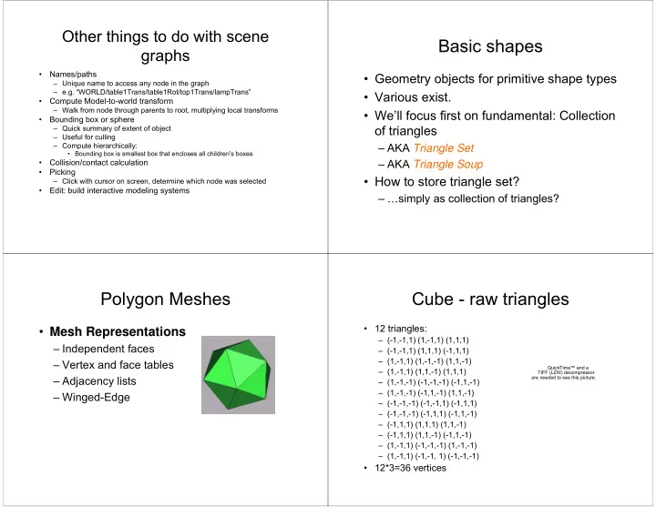
Polygon Meshes

• Mesh Representations

– Independent faces – Vertex and face tables – Adjacency lists – Winged-Edge

• 12 triangles:

– (-1,-1,1) (1,-1,1) (1,1,1) – (-1,-1,1) (1,1,1) (-1,1,1) – (1,-1,1) (1,-1,-1) (1,1,-1) – (1,-1,1) (1,1,-1) (1,1,1) – (1,-1,-1) (-1,-1,-1) (-1,1,-1) – (1,-1,-1) (-1,1,-1) (1,1,-1) – (-1,-1,-1) (-1,-1,1) (-1,1,1) – (-1,-1,-1) (-1,1,1) (-1,1,-1) – (-1,1,1) (1,1,1) (1,1,-1) – (-1,1,1) (1,1,-1) (-1,1,-1) – (1,-1,1) (-1,-1,-1) (1,-1,-1) – (1,-1,1) (-1,-1, 1) (-1,-1,-1)

• 12*3=36 vertices

Cube - raw triangles

QuickTime™ and a TIFF (LZW) decompressor are needed to see this picture.

Independent Faces

• Each Face Lists Vertex Coordinates

– Redundant vertices – No topology information

F1 F2 F3 (x1, y1, z1) (x2, y2, z2) (x5, y5, z5) (x3, y3, z3) (x4, y4, z4)

Face Table

F1 F2 F3 (x1, y1, z1) (x2, y2, z2) (x3, y3, z3) (x2, y2, z2) (x4, y4, z4) (x3, y3, z3) (x2, y2, z2) (x5, y5, z5) (x4, y4, z4)

But….

• A cube only has 8 vertices!
• 36 vertices with x,y,z = 36*3 floats = 108 floats.

– Would waste memory to store all 36 vertices – Would be slow to send all 36 vertices to GPU – (Especially when there is additional data per-vertex)

• Usually each vertex is used by at least 3 triangles--often

4 to 6 or more

– Would use 4 to 6 times as much memory as needed, or more

• Instead: Specify vertex data once, then reuse it

– Assign a number to each vertex – Specify triangles using vertex numbers

QuickTime™ and a TIFF (LZW) decompressor are needed to see this picture.

• 8 vertices:

– P0: ( 1,-1, 1) – P1: ( 1,-1,-1) – P2: ( 1, 1,-1) – P3: ( 1, 1, 1) – P4: (-1,-1, 1) – P5: (-1,-1,-1) – P6: (-1, 1,-1) – P7: (-1, 1, 1)

– 8 vertices*3 floats = 24 floats 12 triangles*3 points= 36 integers

Cube - indexed triangles

• 12 triangles:

– P4 P0 P3 – P4 P3 P7 – P0 P1 P2 – P0 P2 P3 – P1 P5 P6 – P1 P6 P2 – P5 P4 P7 – P5 P7 P6 – P7 P3 P2 – P7 P2 P6 – P0 P5 P1 – P0 P4 P5

Indexed Triangle set

• Array of vertex locations, array of Triangle objects:

Point3 vertices[] = { ( 1,-1, 1), ( 1,-1,-1), ( 1, 1,-1), ( 1, 1, 1), (-1,-1, 1), (-1,-1,-1), (-1, 1,-1), (-1, 1, 1)}; class Triangle {short p1, p2, p3) triangles[] = { (4, 0, 3), (4, 3, 7), (0, 1, 2), (0, 2, 3), (1, 5, 6), (1, 6, 2), (5, 4, 7), (5, 7, 6), (7, 3, 2), (7, 2, 6), (0, 5, 1), (0, 4, 5)};

• Triangles refer to each vertex by its index in the vertex array

Vertex & Face Tables

• Each Face Lists Vertex References

– Shared vertices – Still no topology information

F1 F2 F3 (x1, y1, z1) (x2, y2, z2) (x5, y5, z5) (x3, y3, z3) (x4, y4, z4)

Face Table

F1 F2 F3 V1 V2 V3 V2 V4 V3 V2 V5 V4

Vertex Table

V1 V2 V3 V4 V5 x1 y1 z1 x2 y2 z2 x3 y3 z3 x4 y4 z4 x5 y5 z5

QuickTime™ and a TIFF (LZW) decompressor are needed to see this picture.

Benefits of indexing

• Saves memory
• Saves data transmission time
• Save rendering time: lighting calculation can be done

just one for each vertex

• Easy model deformation

– Change vertex position data – Triangles automatically follow

• Topology (point connectivity) separate

from shape (point locations)

(Index vs. pointer)

• Triangle stores indexes into the vertex array.
• Could also use pointer rather than index

– Can be easier to work with – But uses more memory (if pointer is larger than short integer) – Can be fragile: if vertex array is reallocated pointers will dangle

Normals

• Normal = perpendicular to surface
• The normal is essential to lighting

– Shading determined by relation of normal to eye & light

• Collection of triangles with their normals: Facet Normals

– Store & transmit one normal per triangle – Normal constant on each triangle--but discontinuous at triangle edges – Renders as facets – Good for faceted surfaces, such as cube

• For curved surface that is approximated by triangles: Vertex

Normals

– Want normal to the surface, not to the triangle approximation – Don’t want discontinuity: share normal between triangles – Store & transmit one normal per vertex – Each triangle has different normals at its vertices

• Lighting will interpolate (a few weeks)
• Gives illusion of curved surface

Color

• Color analogous to normal

– One color per triangle: faceted – One color per vertex: smooth colors

Indexed Triangle Set with Normals &Colors

• Arrays:

Point3 vertexes[]; Vector3 normals[]; Color colors[]; Triangle triangles[]; int numVertexes, numNormals, numColors, numTriangles;

• Single base class to handle both:

– Facets

• one normal & color per triangle
• numNormals = numColors = numTriangles

– Smooth

• one normal & color per vertex
• numNormals = numColors = numVertexes

Geometry objects base class

• Base class may support an indexed triangle set

class Geometry { Point3 vertices[]; Vector3 normals[]; Color colors[]; Triangle triangles[]; int numVerices,numNormals,numColors,numTriangles; }; class Triangle { int vertexIndices[3]; int normalIndices[3]; int colorIndices[3]; };

• Triangle indices:

– For facet normals, set all three normalIndices of each triangle to same value – For vertex normals, normalIndices will be same as vertexIndices – Likewise for color

Cube class

class Cube(Geometry) { Cube() { numVertices = 8; numTriangles = numNormals = 12; vertices = { ( 1,-1, 1), ( 1,-1,-1), ( 1, 1,-1), ( 1, 1, 1), (-1,-1, 1), (-1,-1,-1), (-1, 1,-1), (-1, 1, 1) }; triangles = { (4, 0, 3), (4, 3, 6), (0, 1, 2), (0, 2, 3), (1, 5, 6), (1, 6, 2), (5, 4, 7), (5, 7, 6), (7, 3, 2), (7, 2, 6), (0, 5, 1), (0, 4, 5) }; normals = { ( 0, 0, 1), ( 0, 0, 1), ( 1, 0, 0), ( 1, 0, 0), ( 0, 0,-1), ( 0, 0,-1), (-1, 0, 0), (-1, 0, 0), ( 0, 1, 0), ( 0, 1, 0), ( 0,-1, 0), ( 0,-1, 0) }; } }

Smooth surfaces

• Tesselation: approximating a smooth surface with a triangle mesh

– Strictly speaking, “tesselation” refers to regular tiling patterns – In computer graphics, often used to mean any triangulation

• E.g. Sphere class fills in triangle set (will get to this shortly…)

class Sphere(Geom) { private: float radius; void tesselate() { vertices = … triangles = … normals=… } public: Sphere(float r) { radius = r;} void setRadius(float r) { radius = r; } }

• Other smooth surface types

– Bezier patch (next week) – NURBS – Subdivision surface – Implicit surface

Drawing the indexed triangle set

• OpenGL supports “vertex arrays”

– This and “vertex buffers” are covered in CSE 781.

• So for Lab 3 and on-ward:

– Use indexed triangle set for base storage – Draw by sending all vertex locations for each triangle:

for (i=0; i<numTriangles; i++) { glVertex3fv(vertexes[triangles[i].p1]); glVertex3fv(vertexes[triangles[i].p2]); glVertex3fv(vertexes[triangles[i].p3]); }

• So we get memory savings in Geometry class
• We don’t get speed savings when drawing.
• Basic indexed triangle set is unstructured: “triangle soup”
• GPUs & APIs usually support slightly more elaborate structures
• Most common: triangle strips, triangle fans

– Store & transmit ordered array of vertex indexes.

• Each vertex index only sent once, rather than 3 or 4-6 or more

– Even better: store vertexes in proper order in array

• Can draw entire strip or fan by just saying which array and how many vertexes
• No need to send indexes at all.

– Can define triangle meshes using adjacent strips

• Share vertexes between strips
• But must use indexes

v0 v1 v2 v4 v6 v8 v7 v5 v3 v0 v1 v2 v3 v4 v5 v6 v7

Triangles, Strips, Fans Model I/O

• Usually have the ability to load data from

some sort of file

• There are a variety of 3D model formats,

but no universally accepted standards

• More formats for mostly geometry (e.g.

indexed triangle sets) than for complete complex scene graphs

• File structure unsurprising: List of vertex data,

list(s) of triangles referring to the vertex data by name or number

Modeling Operations

• Surface of Revolution
• Sweep/Extrude
• Mesh operations

– Stitching – Simplification -- deleting rows or vertices – Inserting new rows or vertices

• Filleting
• Boolean combinations
• Digitize
• Procedural modeling, scripts…

Adjacency Lists

• Store all Vertex, Edge, and Face

Adjacencies

– Efficient topology traversal – Extra storage

F1 F2 F3 V1 V2 V5 V3 V4 E1 E2 E3 E5 E4 E6 E7

V2 V3 E1 E4 E2 E5 E6 F1 F2 V5 V4 V3 V1 E6 E5 E3 E2 F3 F2 F1 V2 V4 V3 E5 E4 E3 F3 F1

Winged Edge

• Adjacency Encoded in Edges

– All adjacencies in O(1) time – Little extra storage (fixed records) – Arbitrary polygons

{Fi} {Vi} {Ei}

1 1 2 2 4

v1 v2 f1 f2 e21 e22 e11 e12

Winged Edge

• Example

F1 F2 F3 (x1, y1, z1) (x2, y2, z2) (x5, y5, z5) (x3, y3, z3) (x4, y4, z4)

Face Table

F1 F2 F3 e1 e3 e5

Vertex Table

V1 V2 V3 V1 V2 x1, y1, z1 x2, y2, z2 x3, y3, z3 x4, y4, z4 x5, y5, z5 E1 E6 E3 E5 E6

Edge Table

E1 E2 E3 E4 E5 E6 E7 V1 V3 V1 V2 V2 V3 V3 V4 V2 V4 V2 V5 V4 V5 E2 E2 E4 E3 E1 E1 E3 E6 E2 E5 E1 E4 E1 E3 E7 E5 E3 E6 E4 E7 E5 E2 E7 E7 E4 E5 E6 E6

11 12 21 22

Modeling Geometry

Surface representation

Large class of surfaces

Traditional splines Implicit surfaces Variational surfaces Subdivision surfaces

Interactive manipulation Numerical modeling

Complex Shapes

Example: Building a hand

Woody’s hand from Pixar’s Toy Story Very, very difficult to avoid seams

No More Seams

Subdivision solves the “stitching” problem

A single smooth surface is defined Example:

Geri’s hand

(Geri’s Game; Pixar)

What is Subdivision?

Subdivision defines a smooth curve or

surface as the limit of a sequence of successive refinements

Why Subdivision?

Many attractive features

Arbitrary topology Scalability, LOD Multiresolution Simple code

Small number of rules

Efficient code

new vertex is computed with a small number of

floating point operations

Subdivision Surfaces

Geri’s Game (1989) : Pixar Animation Studios

Subdivision Surfaces

Approach Limit Curve Surface through an Iterative Refinement

Process.

Refinement 1 Refinement 2 Refinement ∞

Subdivision in 3D

Same approach works in 3D

Refinement

More examples Subdivision Schemes

Basic idea: Start with something coarse, and

refine it into smaller pieces, typically smoothing along the way

Examples:

Subdivision for tessellating a sphere - procedural Subdivision for fractal surfaces – procedural Subdivision with continuity - algebraic

Tessellating a sphere

Various ways to do it A straightforward one:

North & South poles Latitude circles Triangle strips between latitudes Fans at the poles

QuickTime™ and a TIFF (Uncompressed) decompressor are needed to see this picture. QuickTime™ and a TIFF (Uncompressed) decompressor are needed to see this picture. QuickTime™ and a TIFF (Uncompressed) decompressor are needed to see this picture.

Latitude circles

South Pole x z L1 L2 L3 L4 L5 North Pole

π 6

R r

1

r

2

r

3

r

4

r

5

r

2 = Rsin(2π / 6)

z2 = −Rcos(2π / 6)

z2

South Pole North Pole L1 L2 L3 L4 L5 Given: M = # latitude circles R = radius of sphere For ith circle: i from 1 to M r

i = Rsin

iπ M +1 ⎛ ⎝ ⎜ ⎞ ⎠ ⎟ zi = −Rcos iπ M +1 ⎛ ⎝ ⎜ ⎞ ⎠ ⎟

Points on each latitude circle

r

i cos(7π / 4), r i sin(7π / 4), zi

( ) Given ith circle: N = # points in each circle r

i = radius of ith circle

zi = height of ith circle For jth point: j from 0 to N −1 P

ij = r i cos(2π j / N), r i sin(2π j / N), zi

( )

Pi0 x y Pi1 Pi2 Pi3 Pi4 Pi5 Pi6 Pi7

π 4

r

i

P

ij =

Rsin i π M +1 ⎛ ⎝ ⎜ ⎞ ⎠ ⎟ cos j 2π N ⎛ ⎝ ⎜ ⎞ ⎠ ⎟ , Rsin i π M +1 ⎛ ⎝ ⎜ ⎞ ⎠ ⎟ sin j 2π N ⎛ ⎝ ⎜ ⎞ ⎠ ⎟ , −Rcos i π M +1 ⎛ ⎝ ⎜ ⎞ ⎠ ⎟ ⎛ ⎝ ⎜ ⎞ ⎠ ⎟

Normals

For a sphere, normal per vertex is easy!

Radius vector from origin to vertex is

perpendicular to surface

I.e., use the vertex

coordinates as a vector, normalize it

Algorithm Summary

Fill vertex array and normal array:

South pole = (0,0,-R); For each latitude i, for each point j in the circle at that

latitude

Compute coords, put in vertexes

• Put points in vertices[0]..vertices[M*N+1]

North pole = (0,0,R) Normals coords are same as point coords, normalized

Fill triangle array:

N triangles between south pole and Lat 1 2N triangles between Lat 1 & Lat 2, etc. N triangles between Lat M and north pole.

Subdivision Method

Begin with a course approximation to the

sphere, that uses only triangles

Two good candidates are platonic solids with

triangular faces: Octahedron, Isosahedron

They have uniformly sized faces and uniform

vertex degree

Repeat the following process:

Insert a new vertex in the middle of each edge Push the vertices out to the surface of the

sphere

Break each triangular face into 4 triangles

using the new vertices

Octahedron Isosahedron

The First Stage

Each face gets split into 4: Each new vertex is degree 6, original vertices are degree 4

Sphere Subdivision Advantages

All the triangles at any given level are the same size

Relies on the initial mesh having equal sized faces, and

properties of the sphere

The new vertices all have the same degree

Mesh is uniform in newly generated areas

The location and degree of existing vertices does

not change

The only extraordinary points lie on the initial mesh Extraordinary points are those with degree different to the

uniform areas

Example: Catmull-Clark subdivision

16 1 8 3 16 1 16 1 8 3 16 1 4 1 4 1 4 1 4 1 16 9 n 8 3 n 8 3 n 8 3 n 8 3 n 16 1 n 16 1 n 16 1 n 16 1

Types of Subdivision

Interpolating Schemes

Limit Surfaces/Curve will pass through original set

• f data points.

Approximating Schemes

Limit Surface will not necessarily pass through the

• riginal set of data points.

Subdivision in 1D

The simplest example

Piecewise linear subdivision

Subdivision in 1D

A more interesting example

The 4pt scheme

Iterated Smoothing

2 1 3 2 1 2

4 1 4 3 4 3 4 1 P P Q P P Q + = + =

3 2 5 3 2 4

4 1 4 3 4 3 4 1 P P Q P P Q + = + =

1 1 1

4 1 4 3 4 3 4 1 P P Q P P Q + = + =

1 1 2 1 2

4 1 4 3 4 3 4 1

+ + +

+ = + =

i i i i i i

P P Q P P Q Apply Iterated Function System Limit Curve Surface P0 P1 P2 P3 Q0 Q1 Q2 Q3 Q4 Q5

Subdivision in 2D

Quadrilateral

Interpolating : Kobbelt scheme

Subdivision in 2D

Triangular

Approximating : Loop scheme

Terminology

Control point/polygon/surface

The initial vertex/polygon/surface

Odd vertices :

new vertices

Even vertices :

• ld vertices

The Basic Setup (1/3)

All subdivision schemes have 2 steps:

Splitting step (topological rule)

Which introduces midpoints and modifies connectivity

Averaging step (geometric rule)

Which computes the weighted averages indicate by

the equation

The Basic Setup (2/3)

Splitting step (topological rule)

Introduce midpoint and modify connectivity

The Basic Setup (3/3)

Averaging step (geometric rule)

Compute geometry positions

Local linear combinations of points

Approximation vs. interpolation

Interpolating scheme

A new vertex, once computed, is never changed

by successive subdivision

The control points are also points of the limit

surface

Approximating scheme

New vertices are changed by successive

subdivision

Some Conditions (1/5)

Subdivision rules should

be floating point efficient

New vertex should be computed with a small number

• f floating operation

have compact support

Influence of control point is finite

Some Conditions (2/5)

Subdivision rules should

have local definition

Stencil weights only depend on the structure of a small

neighborhood

Some Conditions (3/5)

Subdivision rules should

be affinely invariant

rotation, translation, scaling, shearing

Some Conditions (4/5)

Subdivision rules should

be simple

• nly a small set of different stencils

Ex: Loop scheme

Some Conditions (5/5)

Subdivision rules should

Achieve some order of smoothness

C1 easy, C2 mush harder

The Differencing Mask

Linear subdivision isolates the addition of

new vertices

Differencing repositions vertices Rule is uniform

Extension to Surfaces

Linear subdivision Bilinear subdivision Differencing Two-dimensional differencing Use tensor product

+ +

Surface Example

Linear subdivision + Differencing Subdivision method for curve networks

Example: Circular Torus

Tensions set to zero to produce a circle

Cylinder Example

Open boundary converges to a circle as well

Surface of Revolution

Construct profile curve to define surfaces of

revolution

Optional smoothing

HLSL Shader

[maxvertexcount(10)] void bezier_GS(lineadjfloat4 v[4], inoutLineStream<float4> stream, uniform intsegments = 10) { float4x4 bezierBasis= { { 1, -3, 3, -1 }, { 0, 3, -6, 3 }, { 0, 0, 3, -3 }, { 0, 0, 0, 1 } }; for(inti=0; i<segments; i++) { float t = i / (float) (segments-1); float4 tvec= float4(1, t, t*t, t*t*t); float4 b = mul(bezierBasis, tvec); float4 p = v[0]*b.x+ v[1]*b.y+ v[2]*b.z+ v[3]*b.w; stream.Append(p: SV_POSITION) } CubeMapStream.RestartStrip(); }

From Simon Green’s slides at nVidia

4 control points input, 10 line vertices out. In other words, each line segment is replaced with 9 line segments.

Terrain Map

Height Map

z = f(x, y)

x and y are sampled on a 2D integer grid

Real data : Satellite, Elevation maps Synthetic : Texture map, Noise functions

Terrain Map

Connect samples into a mesh

Procedural Modeling With Fractals

Procedural Modeling

Compute geometry “on-the-fly”

Fractals

Model Natural Phenomena - Self Similarity

Mountains, fire, clouds, etc.

• Scales to infinity

Add or “make up” natural looking details with

mathematical tools

Fractals

“Repetition of form over a variety of scales”

Mandelbrot set, Julia set

Two Fractal Properties

Self-similarity

Two Fractal Properties

Fractal Dimension

Euclidean dimensions : 1, 2, 3, 4, … Fractal : 1.2342, 2.7656 Measure of detail or roughness of a fractal

D = (ln N)/(ln 1/s)

Midpoint Subdivision

Midpoint (recursive) subdivision

Midpoint Subdivision

Brownian Motion

Describes random movement of particles in a gas

• r fluid

Fractional Brownian Motion

Brownian Motion + Fractal Dimension A useful model for natural phenomena

Fractional Brownian Motion

Fractional Brownian Motion

Equations are compute intensive Approximate with “A family of 1D Gaussians ”

Zero mean Standard Deviation : S = k2-iH

H = fractal dimension (roughness)

Fractional Brownian Motion

Fractal dimension = roughness, I.e. H

Fractal Mountains

Recursively subdivide geometry

by random number d:

–dHeight/2 < d < dHeight/2

At each recursion:

dHeight *= 2-r r=1 : self-similar r>1 : large features early r<1 : large features late

A B A B A B

Triangle Subdivision

Subdivide a triangle into 4 triangles at edge

midpoint

Terrain Modeling Criteria

Input

Initial coarse mesh + stochastic parameters

Two criteria

Internal Consistency

Reproducibility : Model is independent of position and

• rientation

Associate “random numbers” to point index

External Consistency

Continuity between adjacent primitives

Quadrilateral Subdivision

Subdivide a quad into 4 quads at edge

midpoints and a new center point.

Diamond-Square Subdivision

Alternate subdivision

Fractal Terrain Mesh Subdivision

Square-square Subdivision

Addresses “creasing problem” (slope

discontinuities)

Subdivide parametric patches

Mesh Subdivision

Displacement is scaled by the recursion level.

| b – a | -rn

When do you stop the recursion?

Pixel resolution

Displace upward, or towards the normal to

the surface?

Mesh Subdivision

External Consistency

Avoid tears between neighboring polygons How do we compute the normals?

Average polygon normals at each vertex. Propagate normals down the recursion Cheaper : use the original mesh normals only

Ridged Fractal Terrains

To create sharp peaks, add an absolute

value and flip the surface upside down.

Or, reflect about a maximum value. Provides a volcano-like effect.

Caldera