Background Large amounts of reciprocal connectivity between cortical - - PowerPoint PPT Presentation

Lateral Interactions and Feedback

Chris Williams

Neural Information Processing School of Informatics, University of Edinburgh

January 15, 2018

1 / 23

Background

◮ Large amounts of reciprocal connectivity between cortical layers ◮ Suggests a role for feedback as well as feed-forward computations ◮ Feedback need not be restricted to notions of selective attention ◮ Feedback influences are natural consequences of probabilistic inference in the graphical models we have studied ◮ Work on computer vision suggests that feedback influences are important for obtaining good performance ◮ See HHH chapter 14

2 / 23

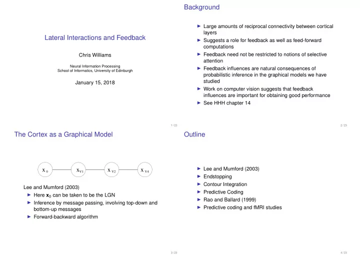
The Cortex as a Graphical Model

x 0 xV1 x V2 x V4

Lee and Mumford (2003) ◮ Here x0 can be taken to be the LGN ◮ Inference by message passing, involving top-down and bottom-up messages ◮ Forward-backward algorithm

3 / 23

Outline

◮ Lee and Mumford (2003) ◮ Endstopping ◮ Contour Integration ◮ Predictive Coding ◮ Rao and Ballard (1999) ◮ Predictive coding and fMRI studies

4 / 23

Lee and Mumford (2003)

◮ Time course of responses of some V1 neurons suggests feedforward response initially, later becomes sensitive to context (e.g. illusory contours in Kanizsa square) ◮ Feedback is particularly important when the input scene is ambiguous, and one may need to entertain multiple competing hypotheses (as for the Kanizsa square)

[Lee and Mumford, 2003] 5 / 23

Example: Endstopping

◮ See e.g. HHH §14.2 ◮ Cell output is reduced when optimal stimulus made longer (reported in 1960’s by Hubel and Wiesel) ◮ Can arise from competitive interactions, e.g. in the sparse coding model ◮ In the example below for the long bar v2 = 0 as it is “explained away” by activation of v1 and v3 ◮ Concept of a “non-classical” receptive field

Figure credit: Hyvärinen, Hurri and Hoyer (2009) 6 / 23

Example: Contour Integration

◮ HHH §14.1 ◮ Consider model with complex cells and countour cells (ICA model) from HHH §12.1 ◮ xk =

i aiksi + nk

◮ s units have sparse priors ◮ nk ∼ N(0, σ2) ◮ Network learns about contour regularities

Figure credit: Hyvärinen, Hurri and Hoyer (2009) 7 / 23

◮ Given input for c we obtain samples from p(s|c) or argmax ˆ s ◮ This gives rise to predictions ˆ c = Aˆ s which are different to c (due to the possibility of noise n) ◮ This is particularly interesting for non-linear feedback (arising from a non-Gaussian prior on s) ◮ Note: can think of integrating out s, this will induce lateral connectivity between the c’s

8 / 23

Figure credit: Hyvärinen, Hurri and Hoyer (2009)

◮ (a) patches, (b) feedforward activations c, (c) ˆ c (after feedback) ◮ Top patch contains aligned Gabors, bottom does not have this alignment ◮ Noise reduction has retained the activations of the co-linear stimuli but suppressed activity that does not fit the learned contour model well

9 / 23

Predictive Coding

◮ Predictive coding (in a general sense) is the idea that the representation of the environment requiers that the brain actively predicts what the sensory input will be, rather than just passively registering it ◮ To an electrical engineer, predictive coding means something like p(x1, x2, . . . , xn) = p(x1)p(x2|x1) . . . p(xn|x1, . . . , xn−1) ◮ What predictive coding is taken to mean in some neuroscience contexts is (roughly) that if there is a top down prediction ˆ ck, then the lower level need only send the prediction error ck − ˆ ck ◮ Question: can you carry out valid inferences passing only these messages? ◮ See HHH §14.3

10 / 23

◮ HHH say (p 317) “the essential difference is in the interpretation of how the abstract quantities are computed and coded in the cortex. In the predictive modelling framework, it is assumed that the prediction errors [ck − ˆ ck] are actually the activities (firing rates) of the neurons on the lower level. This is a strong departure from the framework used in this book, where the ck are considered as the activities of the neurons. Which one of these interpretations is closer to the neural reality is an open question which has inspired some experimental work ...”

11 / 23

Rao and Ballard (1999)

◮ Basically a hierarchical factor analysis model, or tree-structured Kalman filter ◮ u1, u2 and u3 are nearby image patches ◮ At each level there is a predictive estimator (PE) module ◮ R & B need spatial architecture to get interesting effects as the model is linear/Gaussian (cf contour integration) ◮ Top down prediction vtd

i

= Fiw ◮ Error signal vi − vtd

i

(difference between top-down prediction and the actual response) is propagated upwards Ei = 1 σ2 (ui − Givi)T(ui − Givi) + 1 σ2

td

(vi − vtd

i )T(vi − vtd i )

(if vtd

i

= 0 this is simply FA for each patch)

12 / 23

PE PE PE PE

level 0 level 1 level2

3 2 1

u u u

13 / 23

End-stopped responses

short bar long bar

◮ As long edges are more prevalent in natural scenes, the top-down prediction will favour this. ◮ For a long bar, t-d predictions are correct, so errors are close to zero. ◮ For a short bar the t-d predictions are incorrect, so there are more error signals in level 1

14 / 23 Figure credit: Rao and Ballard (1999) 15 / 23

◮ Thus response vi − vtd

i

in a model neuron is stronger for short bars, and decays for longer bars: endstopping (see Fig 3c in R & B) ◮ Similar tuning to experimental data from Bolz and Gilbert (1986), (see Fig 5a in R & B) ◮ The observed endstopping depends on feedback connections (see Fig 5a in R & B) ◮ Other experiments look at predictability of grating patterns

• ver a 3 × 3 set of patches, and observe similar effects

(see Fig 6 in R & B) ◮ Extra-classical RF effects can be seen as an emergent property of the network

16 / 23

3C 5A

Figure credit: Rao and Ballard (1999) 17 / 23

Predictive Coding or Sharpening?

◮ Contour integration a la HHH §14.1 can be called sharpening; increase activity in those aspects of the input that area consistent with the predicted activity, and reduce all other activity. Can lead to an overall reduction in activity ◮ Contrast with predictive coding viewpoint; difference depends on whether unpredicetd activity is noise or signal ◮ See discussion in Murray, Schrater and Kersten (2004)

Figure credit: Murray, Schrater and Kersten (2004) 18 / 23

Predictive coding and fMRI studies

◮ Experiments in Murray, Schrater and Kersten (2004) ◮ Stimuli are lines arranged in 3D, 2D or random configurations ◮ Measure activity in LOC (lateral occipital complex), which has been shown to code for 3D percepts, and V1

Figure credit: Murray, Schrater and Kersten (2004) 19 / 23

Interpreting fMRI studies on predictive coding

◮ fMRI is a very blunt instrument, as every voxel reflects an average of more than 100,000 neurons ◮ Reduced fMRI activity is consistent with sharpening as well as predictive coding ◮ “Predictive coding appears to be at odds with single-neuron recordings indicating that neurons along the ventral pathway respond with vigorous activity ever more complex objects ...” (Koch and Poggio, 1999) ◮ “... what about functional imaging data revealing that particular cortical areas respond to specific image classes.. ? ” (Koch and Poggio, 1999)

20 / 23

◮ Egner et al (2010): “... each stage of the visual cortical hierarchy is thought to harbor two computationally distinct classes of processing unit: representational units that encode the conditional probability of a stimulus (“expectation”) [..]; and error units that encode the mismatch between predictions and bottom up evidence (“surprise”), and forward this prediction error to the next higher level ...” ◮ Need more clarity on how the brain is meant to be implementing belief propagation ...

21 / 23

References

◮ Egner, T., Monti, J. M., Summerfield, C. Expectation and Surprise Determine Neural Population Responses in the Ventral Visual Stream. J. Neurosci. 30(49) 16601-16608 (2010) ◮ Koch, C. and Poggio, T. Predicting the Visual World: Silence is Golden. Nature Neurosci. 2(1) 9-10 (1999) ◮ Lee, T-S., Mumford, D. Hierarchical Bayesian inference in the visual cortex, J. Opt. Soc. America 20(7) 1434-1448 (2003) ◮ Murray, S. O., Schrater, P . and Kersten D. Perceptual grouping and the interactions between visual cortical

• areas. Neural Networks 17 695-705 (2004)

◮ Rao, R. P . N., Ballard, D. H. Predictive coding in the visual cortex: a functional interpretation of some extra-classical receptive-field effects, Nature Neurosci. 2(1) 79-87 (1999)

22 / 23