
SLIDE 1
ARMAX Models
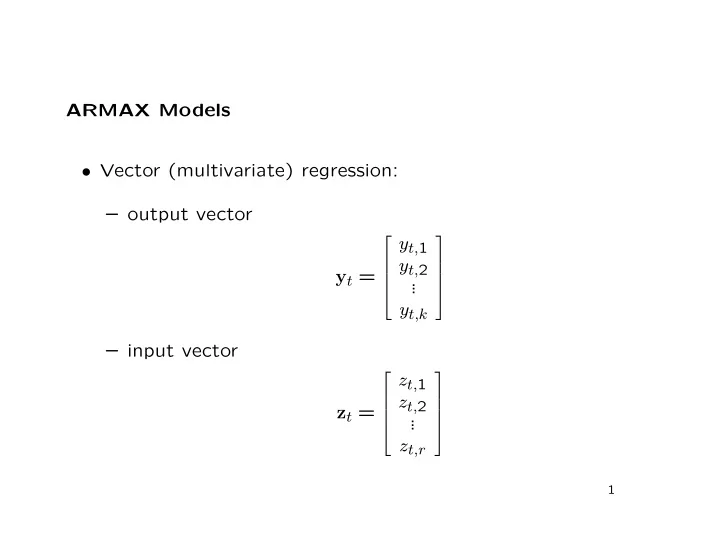
- Vector (multivariate) regression:
B = Y Z Z Z where y z 1 1 y z - - PowerPoint PPT Presentation
ARMAX Models Vector (multivariate) regression: output vector y t, 1 y t, 2 y t = . . . y t,k input vector z t, 1 z t, 2 z t = . . .