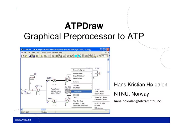
ATPDraw Graphical Preprocessor to ATP Hans Kristian Hidalen NTNU, - PowerPoint PPT Presentation

1 ATPDraw Graphical Preprocessor to ATP Hans Kristian Høidalen NTNU, Norway hans.hoidalen@elkraft.ntnu.no

2 Contents • Introduction • Overview of ATPDraw functionality • Examples • Latest news in version 5.0-5.4

3 Introduction • ATPDraw is a graphical, mouse-driven, dynamic preprocessor to ATP on the Windows platform • Handles node names and creates the ATP input file based on ”what you see is what you get” • Freeware • Supports – All types of editing operations – ~100 standard components – ~60 TACS components – MODELS – $INCLUDE and User Specified Components – Groups

4 Introduction- ATPDraw history • Simple DOS version – Leuven EMTP Centre, fall meeting 1991, 1992 • Extended DOS versions, 1994-95 • Windows version 1.0, July 1997 – Line/Cable modelling program ATP_LCC BPA Sponsored – User Manual • Windows version 2.0, Sept. 1999 – MODELS, more components (UM, SatTrafo ++) – Integrated line/cable support (Line Constants + Cable Parameters)

5 Introduction- ATPDraw history • Windows version 3, Dec. 2001 – Grouping/Compress – Data Variables, $Parameter + PCVP – LCC Verify + Cable Constants – BCTRAN – User Manual @ version 3.5 • Windows version 4, July 2004 – Line Check – Hybrid Transformer model – Zigzag Saturable transformer • Windows version 5, Oct. 2006 – Vector graphics, multi-phase nodes, interactive Models integration, files in memory

6 ATPDraw functionality Main menu Tool bar Circuit Header, map circuit file name Component Circuit selection menu windows Circuit under construction

7 ATPDraw Component dialog Node names Editable Red=User Spec. data values Used for sorting Label on Windows screen clipboard Comment in support ATP file Branch Component output not to ATP Edit local High definitions precision Icon/help/ Local help pos/name/ F1=Global help units

8 I ATPDraw capability V I I I Los Banos 30050 3 LCC 1 LB - Mid LCC 3 LCC V LCC 1 V I I Gates 30055 V I I V V V I V I I I I I t I I • 30.000 nodes V I I I I I I LCC LCC LCC 3 • 10.000 components LCC LCC LCC Diab lo Canyon 2 LCC LCC 0 30057 V LCC LCC UI I LCC LCC • 10.000 connections UI I I V MIDWAY I UI I I UI 30060 V • 1.000 text strings 2 1 3 I I I LCC LCC • Up to 64 data and 32 nodes per component LCC LCC LCC I 3 LUGO LCC 24086 1 • Up to 26 phases per node (A..Z extension) I 2 LCC 1 I LCC 2 V V 1 I • 21 phases in lines&cables module 2 I LCC I VINCENT LCC 24156 LCC LCC • Unlimited grouping hierarchy 2 3 V MIRA LOMA • 100 UnDo/ReDo steps 24092 LCC 24138 SERRANO LCC LCC VALLEY 24151 V LCC V

9 ATPDraw Edit options • Multiple documents – several circuit windows – large circuit windows (map+scroll) – grid snapping • Circuit editing – Copy/Paste, Export/Import, Rotate/Flip, Undo/Redo (100), Zoom, Compress/Extract – Windows Clipboard: Circuit drawings, icons, text, circuit data • Text editor – Viewing and editing of ATP, LIS, model files, and help files • Help file system – Help on ATPDraw functionality, all components, and MODELS

10 All standard components Prob es & 3-phase UserSpec Branch L. lump L. distr Switches NonLin Machines Trafos Models TACS Devices Fortran V R(i) n 1 : LIB SM T Gdu f F P S dt K + 50 59 v - if 51 n 1 : T SM Math P S * + I Y Y + Vf - 60 - x 52 x T LINE y + T Z-T P S y SM + 61 R(t) ω LINE FreqComp M T Z-MT sin S Sampl Y IM T rack U SAT ω x 53 62 MOV |x| LINE cos HFS C Z-T T H L MIN IM NEG tan U(0) MAX CIGRE MOV H I ω LOAD 54 63 InitCond exp cotan + M T S i(0) TACS BCT CIGRE MIN SP INIT MAX + LOAD Y log asin ω 55 64 STAT C log10 acos RLC Line/Cab G(s) DC ACC XFMR SY ST ω 56 65 Y RAD atan G(s) F(s|z) + Excit ABC DEF RMS DEG sinh 57 LCC K 66 Windsyn LCC + s RND cosh G u Logic Torque K·s 58 tanh H K 1+T·s K·s 1+T·s x=y x x x y x y y y

11 ATPDraw node naming • "What you see is what you get" • Connected nodes automatically get the same name – Direct node overlap nodes connected nodes overlap – Positioned on connection • Warnings in case of duplicates and disconnections • 3-phase and n -phase nodes Connection – Extensions A..Z added automatically 1 – Objects for transposition and splitting ABC – Connection between n - and single Transposition Splitter phase

12 User’s manual • Documents version 3.5 of ATPDraw (246 pages), pdf • Written by Laszlo Prikler and H. K. Høidalen • Content – Intro: To ATP and ATPDraw + Installation – Introductory manual: Mouse+Edit, MyFirstCircuit – Reference manual: All menus and components – Advanced manual: Grouping/LCC/Models/BCTRAN + create new components – Application manual: 9 real examples

6 54 5 54 4 54 x y 3 x y T 54 K Freq 2 T 54 1 54 • Increased circuit readability 6-phase • Multi-phase connections T - + x y Freq x y 58 G u Angle T 180 T T - T Example 1 + T 2 5 6 3 4 1 13

14 Example 2 • Multi-phase groups POS + T - T + PULSE 1 3 AC AC POS - LCC Y Y NEG SAT NEG PULSE 1 4 3 6 5 2 6-phase • New component: Collector

15 Example 3 MODEL FOURIER INPUT X --input signal to be transformed DATA FREQ {DFLT:50} --power frequency n {DFLT:26} --number of harmonics to calculate OUTPUT absF[1..26], angF[1..26],F0 --DFT signals VAR absF[1..26], angF[1..26],F0,reF[1..26], imF[1..26], i,NSAMPL,OMEGA,D,F1,F2,F3,F4 • Multi-phase Models 5 uH 5 mF UI U(0) + M MODEL Cable 0.0265 V Y fourier Y Y Z SAT SAT 1 Diode 132/11.3 Zig-zag HVBUS bridges Regulation transformers 5 uH I 5 mF Y Y ZN0d11y0 transformers SAT UI 10.7/0.693 kV 132 kV 22.2 mH 11.3/10.6 kV U(0) + Cable 0.0265 V Y Y Y Z 20 SAT SAT 16 12 • New Model probe 8 4 0 0.02 0.03 0.04 0.05 0.06 0.07 0.08 0.09 [s] 0.10 (f ile Exa_14.pl4; x-v ar t) m:X0027E m:X0027G m:X0027V m:X0027Y

16 Example 4 • Lightning study • JMarti lines • Simple Bergeron lines in sub-station • Flashover char. In MODELS LINE1 U H V LINE2 L_imp I TOP TWR4 V LCC LCC LCC LCC LCC LCC PT1 A V t t t t TR400 V TR t t t I I I R(i) R(i) R(i)

Transformer modeling SAT Y XFMR Z Y BCT • Saturable Transformer Y • Hybrid Transformer • BCTRAN 17

18 Saturable transformer • Zigzag supported Zig-zag transformers ZN0d11y0 10.7/0.693 kV 5 uH V Zdy UI -12 U(0) 26.5mohm 5 mF + Cable V Y Y Y Z SAT SAT 5 uH V Zdy UI -6 U(0) 26.5mohm 5 mF + Cable V Y Y Y Z SAT SAT 5 uH V transformers 11.3/10.6 kV Ydy UI 132 kV 132/11.3 U(0) 26.5mohm 5 mF + Cable V Y Y Y Y Y Y SAT SAT SAT 22.2 mH 5 uH V Zdy UI +6 U(0) 26.5mohm 5 mF + Cable V Y Y Y Z SAT SAT 5 uH V Zdy UI +12 U(0) 26.5mohm 5 mF + Cable V Y Y Y Z SAT SAT

19 BCTRAN • Automatic inclusion of external magnetization characteristic XFMR V V V Y XFMR I 16 kV BCT V V Y BCTRAN I 80 [A] 50 20 -10 -40 -70 0.00 0.02 0.04 0.06 0.08 [s] 0.10 (f ile Exa_16.pl4; x-v ar t) c:X0004A-LV_XA c:X0004A-LV_BA

20 Hybrid transformer • Four separate parts connected – Leakage: A-matrix; Auto, Y, D with all phase shifts – Winding resistance: Frequency dep. with Foster equiv. – Core: Topological correct core: Frolich equation, relative dimensions. Connected at n +1 winding at core surface. – Capacitance C HA-Xa /2 6 C H-GND /2 C X-GND /2 L 3 N H : N X N X : N X a A L 4 R H ( f ) R X ( f ) C HA-HB /2 Z l ’ a’ Z y A’ C HA-HB /2 C H-GND /2 N H : N X N X : N X b B L 3 R H ( f ) R X ( f ) C HB-HC /2 Z l ’ b’ Z y B’ C H-GND /2 C HB-HC /2 N H : N X N X : N X c C R H ( f ) R X ( f ) Z l L 4 ’ c’ C’ L 3 C H-GND /2 C X-GND /2

21 Hybrid cont. • Design, test report, or typical values Open and short Typical values from Winding geometry circuit test report text books

22 Line/Cable modeling • Line/Cable Constants, Cable Parameters – Bergeron, PI, JMarti, Semlyen, Noda(?) • View – Cross section, grounding • Verify log(| Z |) 3.9 – Frequency response, power frequency params. 2.7 • Line Check 1.5 - Power freq. test of line/cable sections log(freq) 0.4 0.0 2.0 4.0 6.0

23 Example • Double circuit case (420 kV + 145 kV) 12 m 11 m 11 m 4.5 m 9.6 m 4.5 m4.5 m 3.8 m 18.6 m 11 m 35.5 m Test type Circuit Positive sequence system Zero sequence system Z [ Ω /km] Z [ Ω /km] [kV] C [nF/km] C [nF/km] Benchmark data 420 0.02+j0.29 12.8 0.19+j0.71 9.3 50 Hz, 100 Ω m 145 0.06+j0.38 9.7 0.25+j0.80 6.7 Individual testing 420 0.02+j0.29 12.8 0.18+j0.71 9.3 Bergeron model 145 0.06+j0.38 9.7 0.25+j0.80 6.9

Creating the Bergeron model 24

Testing the Bergeron model • Line Model Frequency scan. Model OK for 50 Hz. 25

26 Line Check • The user selects a group in the circuit • ATPDraw identifies the inputs and outputs (user modifiable)

27 Line Check cont. • ATPDraw reads the lis-file and calculates the series impedance and shunt admittance