Artificial Intelligence: Methods and Applications Lecture 4: Path - - PDF document

Artificial Intelligence: Methods and Applications

Lecture 4: Path planning Henrik Björklund

Umeå University

• 28. November 2012

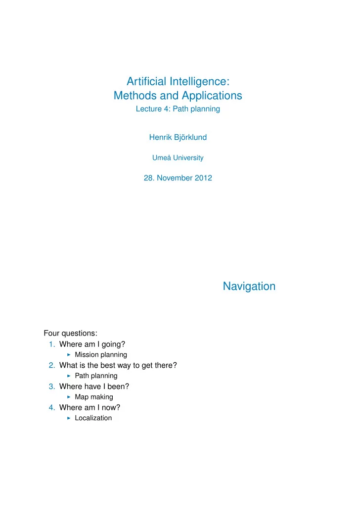
Navigation

Four questions:

• 1. Where am I going?

◮ Mission planning

• 2. What is the best way to get there?

◮ Path planning

• 3. Where have I been?

◮ Map making

• 4. Where am I now?

◮ Localization

Spatial memory

To know what is the best way to a goal, we have to have a world model. World model = Spatial memory The spatial memory supports

◮ Path planning ◮ Attention (what to look for next) ◮ Reasoning (is the mountain to steep?) ◮ Information collection

Spatial memory can provide both geometry and miscellaneous information about places and objects.

Two forms of spatial memory

◮ Based on landmarks (qualitative / topological / route) ◮ Based on maps (quantitative / metric / layout)

Topological spatial memory

◮ Expresses space in terms of relationships between landmarks and

gateways

◮ Orientation clues are egocentric - representation depends on the

perspective of the robot

◮ Cannot in general be used to generate metric representations

Metric spatial memory

◮ Expresses space in terms of a metric map ◮ Not dependen on the perspective of the robot ◮ Can be used to generate topological representations

Why don’t we simply always use metric representations?

Landmarks

One or more perceptually distinctive features on an object or location.

◮ Natural landmarks are not explicitly intended for navigation ◮ Artificial landmarks are explicitly intended for navigation

Desirable characteristics:

◮ Recognizable

◮ From sufficiently long range ◮ From different viewpoints

◮ Identifiable

◮ Global, or at least local, uniqueness

◮ Support task dependent activities

Topological path planning methods

◮ Relational

◮ Spatial memory is based on landmarks ◮ World model is a graph (topological map, relational graph) ◮ Use graph-theoretic algorithms for path planning

◮ Associative

◮ Spacial memory based on viewpoints ◮ Good for retracing one’s steps

Relational graphs Relational graphs R1 R2 R3 R4 R5 G1 G2 G3 G4 G5 G6 G7 G8 G9

Relational graphs

R1 R2 R3 R4 R5 G1 G2 G3 G4 G5 G6 G7 G8 G9

Relational graphs

R1 R2 R3 R4 R5 G1 G2 G3 G4 G5 G6 G7 G8 G9

Relational graphs

R1 R2 R3 R4 R5 G1 G2 G3 G4 G5 G6 G7 G8 G9

Problems with relational graphs

◮ The graph is not coupled with information on how to get from one node to

another

◮ Dead reckoning accumulates uncertainty ◮ Possible solution: add localization to landmarks ◮ Distinctive places

Path planning with relational graphs

◮ Assign behaviors (Local Control Strategies) to edges ◮ Use graph search (i.e., Dijkstras algorithm) to find the best path

A note on localization

What is our primary technology for localization today? Yes: GPS Why don’t we always use it?

◮ Doesn’t work at all on Mars or in the deep blue sea ◮ Doesn’t work that well indoors (especially not under ground) ◮ Sensitive to weather conditions, radio signals, etc.

Associative methods

◮ Spatial memory is a series of remembered viewpoints ◮ Each viewpoint is labeled with a location ◮ Good for retracing steps - not real planning ◮ Couples perception with action

Two methods

◮ Visual homing

◮ Bees navigate to their hives by a series of image signatures which are

locally distinctive

◮ QualNav

◮ Works best outdoors ◮ The world is divided into orientational regions based on perceptual events

caused by landmark pair bounaries

◮ The set of angles to the landmarks is called a viewframe and is used to

navigate within an orientational region

Door from the front Door from the front

Door from the front Door from the front

Door from the right Door from the right

Door from the right Door from the right

Metric path planning

◮ Representation is independent of view, viewpoint, and position ◮ Distance is important ◮ Graph or network algorithms ◮ Wavefront and other graphics-derived algorithms

Metric path planning

◮ Path planning assumes an a priori map of relevant aspects

◮ Relevant: occupied or empty, task relevance ◮ Only as good as the quality of the map permits

◮ Determine a path from one point to another

◮ Generally, we want the best path ◮ Best for what measure?

Cspace

◮ World space: the physical world that the robot functions in (typically

3-dimensional)

◮ In 3-dimensional space, we typically need to keep track of 6 degrees of

freedom (DOFs)

◮ Configuration space (Cspace) is the representation the robot actually

uses

◮ Simplifying assumptions ◮ For a low, flat vacuum robot functioning indoors, we typically only need 3

DOFs (2D position plus heading)

Cspace representations

A Cspace representation should be well suited for computer storage and for rapid execution of path planning algorithms. It should contain all the details that are relevant to the robots operations, but no more. Three common types are

◮ Meadow Maps ◮ Regular grids (and quad trees) ◮ Generalized Voronoi Graphs

Meadow maps Meadow maps

Meadow maps Meadow maps

Meadow maps Meadow maps

Problems with meadow maps

◮ What are the generated pahs like?

◮ Often jagged and a bit on the long side ◮ Path relaxation helps

◮ Can meadow maps be created using sensor data?

◮ What about noice? ◮ How does the robot recognize the right corners and edges? ◮ Computationally heavy

Grids and quad trees

Grids and quad trees Grids and quad trees

Grids and quad trees Grids and quad trees

Grids and quad trees Voronoi graphs

Voronoi graphs A∗ on a grid

A∗ on a grid A∗ on a grid

A∗ on a grid A∗ on a grid

A∗ on a grid A∗ on a grid

A∗ on a grid A∗ on a grid

A∗ on a grid A∗ on a grid

A∗ on a grid A∗ on a grid

A∗ on a grid A∗ on a grid

A∗ on a grid A∗ on a grid

A∗ on a grid A∗ on a grid

Wavefront planners

◮ General idea: Consider the Cspace to be a conductive material with heat

radiating out from the initial node

◮ Well-suited for grid Cspace ◮ Results in a map that looks like a potential field ◮ Optimal path from all grid elements to the goal can be easily computed ◮ Can handle different terrains:

◮ Obstacle: zero conductivity ◮ Rough terrain: low conductivity ◮ Easy terrain: high conductivity

Path planning and reactive execution

Two types of problems:

◮ Subgoal obsession.

◮ Termination conditions: approximate subpath termination ◮ Compute all paths in advance (implicit in wavefront planners)

◮ Incorrect maps

◮ Opportunistic replanning ◮ Compute all paths in advance