Announcements CS 188: Artificial Intelligence Spring 2011 W4 out, - - PDF document

1

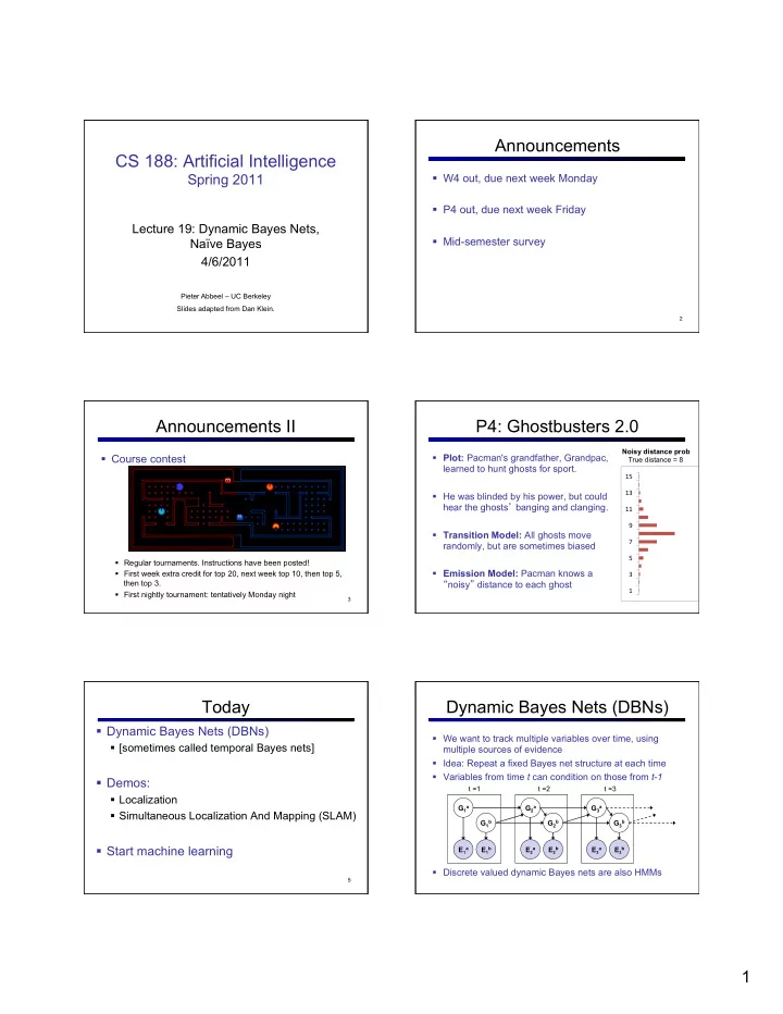
CS 188: Artificial Intelligence

Spring 2011

Lecture 19: Dynamic Bayes Nets, Naïve Bayes 4/6/2011

Pieter Abbeel – UC Berkeley Slides adapted from Dan Klein.

Announcements

§ W4 out, due next week Monday § P4 out, due next week Friday § Mid-semester survey

2

Announcements II

§ Course contest

§ Regular tournaments. Instructions have been posted! § First week extra credit for top 20, next week top 10, then top 5, then top 3. § First nightly tournament: tentatively Monday night

3

P4: Ghostbusters 2.0

§ Plot: Pacman's grandfather, Grandpac, learned to hunt ghosts for sport. § He was blinded by his power, but could hear the ghosts’ banging and clanging. § Transition Model: All ghosts move randomly, but are sometimes biased § Emission Model: Pacman knows a “noisy” distance to each ghost

1 3 5 7 9 11 13 15 Noisy distance prob True distance = 8

Today

§ Dynamic Bayes Nets (DBNs)

§ [sometimes called temporal Bayes nets]

§ Demos:

§ Localization § Simultaneous Localization And Mapping (SLAM)

§ Start machine learning

5

Dynamic Bayes Nets (DBNs)

§ We want to track multiple variables over time, using multiple sources of evidence § Idea: Repeat a fixed Bayes net structure at each time § Variables from time t can condition on those from t-1 § Discrete valued dynamic Bayes nets are also HMMs

G1

a

E1a E1b G1

b

G2

a

E2a E2b G2

b

t =1 t =2 G3

a

E3a E3b G3

b

t =3

2

Exact Inference in DBNs

§ Variable elimination applies to dynamic Bayes nets § Procedure: “unroll” the network for T time steps, then eliminate variables until P(XT|e1:T) is computed § Online belief updates: Eliminate all variables from the previous time step; store factors for current time only

7

G1

a

E1a E1b G1

b

G2

a

E2a E2b G2

b

G3

a

E3a E3b G3

b

t =1 t =2 t =3 G3

b

DBN Particle Filters

§ A particle is a complete sample for a time step § Initialize: Generate prior samples for the t=1 Bayes net § Example particle: G1

a = (3,3) G1 b = (5,3)

§ Elapse time: Sample a successor for each particle § Example successor: G2

a = (2,3) G2 b = (6,3)

§ Observe: Weight each entire sample by the likelihood of the evidence conditioned on the sample § Likelihood: P(E1

a |G1 a ) * P(E1 b |G1 b )

§ Resample: Select prior samples (tuples of values) in proportion to their likelihood

8

[Demo]

DBN Particle Filters

§ A particle is a complete sample for a time step § Initialize: Generate prior samples for the t=1 Bayes net § Example particle: G1

a = (3,3) G1 b = (5,3)

§ Elapse time: Sample a successor for each particle § Example successor: G2

a = (2,3) G2 b = (6,3)

§ Observe: Weight each entire sample by the likelihood of the evidence conditioned on the sample § Likelihood: P(E1

a |G1 a ) * P(E1 b |G1 b )

§ Resample: Select prior samples (tuples of values) in proportion to their likelihood

9

Trick I to Improve Particle Filtering Performance: Low Variance Resampling

§ Advantages:

§ More systematic coverage of space of samples § If all samples have same importance weight, no samples are lost § Lower computational complexity

§ If no or little noise in transitions model, all particles will start to coincide à regularization: introduce additional (artificial) noise into the transition model

Trick II to Improve Particle Filtering Performance: Regularization

SLAM

§ SLAM = Simultaneous Localization And Mapping

§ We do not know the map or our location § Our belief state is over maps and positions! § Main techniques: Kalman filtering (Gaussian HMMs) and particle methods

§ [DEMOS]

DP-SLAM, Ron Parr

3

Robot Localization

§ In robot localization:

§ We know the map, but not the robot’s position § Observations may be vectors of range finder readings § State space and readings are typically continuous (works basically like a very fine grid) and so we cannot store B(X) § Particle filtering is a main technique

§ [Demos]

Global-floor

SLAM

§ SLAM = Simultaneous Localization And Mapping

§ We do not know the map or our location § State consists of position AND map! § Main techniques: Kalman filtering (Gaussian HMMs) and particle methods

15

Particle Filter Example

map of particle 1 map of particle 3 map of particle 2 3 particles

SLAM

§ DEMOS

§ fastslam.avi, visionSlam_heliOffice.wmv

Further readings

§ We are done with Part II Probabilistic Reasoning § To learn more (beyond scope of 188):

§ Koller and Friedman, Probabilistic Graphical Models (CS281A) § Thrun, Burgard and Fox, Probabilistic Robotics (CS287)

Part III: Machine Learning

§ Up until now: how to reason in a model and how to make optimal decisions § Machine learning: how to acquire a model

• n the basis of data / experience

§ Learning parameters (e.g. probabilities) § Learning structure (e.g. BN graphs) § Learning hidden concepts (e.g. clustering)

4

Machine Learning Today

§ An ML Example: Parameter Estimation

§ Maximum likelihood § Smoothing

§ Applications § Main concepts § Naïve Bayes

Parameter Estimation

§ Estimating the distribution of a random variable § Elicitation: ask a human (why is this hard?) § Empirically: use training data (learning!)

§ E.g.: for each outcome x, look at the empirical rate of that value: § This is the estimate that maximizes the likelihood of the data

§ Issue: overfitting. E.g., what if only observed 1 jelly bean?

r g g

r g g r g g r g g r g g r g g

Estimation: Smoothing

§ Relative frequencies are the maximum likelihood estimates § In Bayesian statistics, we think of the parameters as just another random variable, with its own distribution

????

Estimation: Laplace Smoothing

§ Laplace’s estimate:

§ Pretend you saw every outcome

• nce more than you actually did

§ Can derive this as a MAP estimate with Dirichlet priors (see cs281a)

H H T

Estimation: Laplace Smoothing

§ Laplace’s estimate (extended):

§ Pretend you saw every outcome k extra times § What’s Laplace with k = 0? § k is the strength of the prior

§ Laplace for conditionals:

§ Smooth each condition independently:

H H T

Example: Spam Filter

§ Input: email § Output: spam/ham § Setup:

§ Get a large collection of example emails, each labeled “spam” or “ham” § Note: someone has to hand label all this data! § Want to learn to predict labels of new, future emails

§ Features: The attributes used to

make the ham / spam decision § Words: FREE! § Text Patterns: $dd, CAPS § Non-text: SenderInContacts § …

Dear Sir. First, I must solicit your confidence in this transaction, this is by virture of its nature as being utterly confidencial and top

• secret. …

TO BE REMOVED FROM FUTURE MAILINGS, SIMPLY REPLY TO THIS MESSAGE AND PUT "REMOVE" IN THE SUBJECT. 99 MILLION EMAIL ADDRESSES FOR ONLY $99 Ok, Iknow this is blatantly OT but I'm beginning to go insane. Had an old Dell Dimension XPS sitting in the corner and decided to put it to use, I know it was working pre being stuck in the corner, but when I plugged it in, hit the power nothing happened.

5

Example: Digit Recognition

§ Input: images / pixel grids § Output: a digit 0-9 § Setup:

§ Get a large collection of example images, each labeled with a digit § Note: someone has to hand label all this data! § Want to learn to predict labels of new, future digit images

§ Features: The attributes used to make the

digit decision § Pixels: (6,8)=ON § Shape Patterns: NumComponents, AspectRatio, NumLoops § … 1 2 1 ??

Other Classification Tasks

§ In classification, we predict labels y (classes) for inputs x § Examples:

§ Spam detection (input: document, classes: spam / ham) § OCR (input: images, classes: characters) § Medical diagnosis (input: symptoms, classes: diseases) § Automatic essay grader (input: document, classes: grades) § Fraud detection (input: account activity, classes: fraud / no fraud) § Customer service email routing § … many more

§ Classification is an important commercial technology!

Important Concepts

§ Data: labeled instances, e.g. emails marked spam/ham

§ Training set § Held out set § Test set

§ Features: attribute-value pairs which characterize each x § Experimentation cycle

§ Learn parameters (e.g. model probabilities) on training set § (Tune hyperparameters on held-out set) § Compute accuracy of test set § Very important: never “peek” at the test set!

§ Evaluation

§ Accuracy: fraction of instances predicted correctly

§ Overfitting and generalization

§ Want a classifier which does well on test data § Overfitting: fitting the training data very closely, but not generalizing well § We’ll investigate overfitting and generalization formally in a few lectures

Training Data Held-Out Data Test Data

Bayes Nets for Classification

§ One method of classification:

§ Use a probabilistic model! § Features are observed random variables Fi § Y is the query variable § Use probabilistic inference to compute most likely Y

§ You already know how to do this inference

Simple Classification

§ Simple example: two binary features

M S F direct estimate Bayes estimate (no assumptions) Conditional independence

+

General Naïve Bayes

§ A general naive Bayes model: § We only specify how each feature depends on the class § Total number of parameters is linear in n

Y F1 Fn F2 |Y| parameters n x |F| x |Y| parameters |Y| x |F|n parameters

6

Inference for Naïve Bayes

§ Goal: compute posterior over causes

§ Step 1: get joint probability of causes and evidence § Step 2: get probability of evidence § Step 3: renormalize

+

General Naïve Bayes

§ What do we need in order to use naïve Bayes?

§ Inference (you know this part)

§ Start with a bunch of conditionals, P(Y) and the P(Fi|Y) tables § Use standard inference to compute P(Y|F1…Fn) § Nothing new here

§ Estimates of local conditional probability tables

§ P(Y), the prior over labels § P(Fi|Y) for each feature (evidence variable) § These probabilities are collectively called the parameters of the model and denoted by θ § Up until now, we assumed these appeared by magic, but… § …they typically come from training data: we’ll look at this now

A Digit Recognizer

§ Input: pixel grids § Output: a digit 0-9

Naïve Bayes for Digits

§ Simple version:

§ One feature Fij for each grid position <i,j> § Possible feature values are on / off, based on whether intensity is more or less than 0.5 in underlying image § Each input maps to a feature vector, e.g. § Here: lots of features, each is binary valued

§ Naïve Bayes model: § What do we need to learn?

Examples: CPTs

1 0.1 2 0.1 3 0.1 4 0.1 5 0.1 6 0.1 7 0.1 8 0.1 9 0.1 0.1 1 0.01 2 0.05 3 0.05 4 0.30 5 0.80 6 0.90 7 0.05 8 0.60 9 0.50 0.80 1 0.05 2 0.01 3 0.90 4 0.80 5 0.90 6 0.90 7 0.25 8 0.85 9 0.60 0.80

Parameter Estimation

§ Estimating distribution of random variables like X or X | Y § Empirically: use training data

§ For each outcome x, look at the empirical rate of that value: § This is the estimate that maximizes the likelihood of the data

§ Elicitation: ask a human!

§ Usually need domain experts, and sophisticated ways of eliciting probabilities (e.g. betting games) § Trouble calibrating

r g g

7

A Spam Filter

§ Naïve Bayes spam filter § Data:

§ Collection of emails, labeled spam or ham § Note: someone has to hand label all this data! § Split into training, held-

• ut, test sets

§ Classifiers

§ Learn on the training set § (Tune it on a held-out set) § Test it on new emails

Dear Sir. First, I must solicit your confidence in this transaction, this is by virture of its nature as being utterly confidencial and top

• secret. …

TO BE REMOVED FROM FUTURE MAILINGS, SIMPLY REPLY TO THIS MESSAGE AND PUT "REMOVE" IN THE SUBJECT. 99 MILLION EMAIL ADDRESSES FOR ONLY $99 Ok, Iknow this is blatantly OT but I'm beginning to go insane. Had an old Dell Dimension XPS sitting in the corner and decided to put it to use, I know it was working pre being stuck in the corner, but when I plugged it in, hit the power nothing happened.

Naïve Bayes for Text

§ Bag-of-Words Naïve Bayes:

§ Predict unknown class label (spam vs. ham) § Assume evidence features (e.g. the words) are independent § Warning: subtly different assumptions than before!

§ Generative model § Tied distributions and bag-of-words

§ Usually, each variable gets its own conditional probability distribution P(F|Y) § In a bag-of-words model

§ Each position is identically distributed § All positions share the same conditional probs P(W|C) § Why make this assumption?

Word at position i, not ith word in the dictionary!

Example: Spam Filtering

§ Model: § What are the parameters? § Where do these tables come from?

the : 0.0156 to : 0.0153 and : 0.0115

• f : 0.0095

you : 0.0093 a : 0.0086 with: 0.0080 from: 0.0075 ... the : 0.0210 to : 0.0133

• f : 0.0119

2002: 0.0110 with: 0.0108 from: 0.0107 and : 0.0105 a : 0.0100 ... ham : 0.66 spam: 0.33

Spam Example

Word P(w|spam) P(w|ham) Tot Spam Tot Ham (prior) 0.33333 0.66666

• 1.1
• 0.4

Gary 0.00002 0.00021

• 11.8
• 8.9

would 0.00069 0.00084

• 19.1
• 16.0

you 0.00881 0.00304

• 23.8
• 21.8

like 0.00086 0.00083

• 30.9
• 28.9

to 0.01517 0.01339

• 35.1
• 33.2

lose 0.00008 0.00002

• 44.5
• 44.0

weight 0.00016 0.00002

• 53.3
• 55.0

while 0.00027 0.00027

• 61.5
• 63.2

you 0.00881 0.00304

• 66.2
• 69.0

sleep 0.00006 0.00001

• 76.0
• 80.5

P(spam | w) = 98.9

Example: Overfitting

2 wins!!

Example: Overfitting

§ Posteriors determined by relative probabilities (odds ratios):

south-west : inf nation : inf morally : inf nicely : inf extent : inf seriously : inf ...

What went wrong here?

screens : inf minute : inf guaranteed : inf $205.00 : inf delivery : inf signature : inf ...

8

Generalization and Overfitting

§ Relative frequency parameters will overfit the training data!

§ Just because we never saw a 3 with pixel (15,15) on during training doesn’t mean we won’t see it at test time § Unlikely that every occurrence of “minute” is 100% spam § Unlikely that every occurrence of “seriously” is 100% ham § What about all the words that don’t occur in the training set at all? § In general, we can’t go around giving unseen events zero probability

§ As an extreme case, imagine using the entire email as the only feature

§ Would get the training data perfect (if deterministic labeling) § Wouldn’t generalize at all § Just making the bag-of-words assumption gives us some generalization, but isn’t enough

§ To generalize better: we need to smooth or regularize the estimates

Estimation: Smoothing

§ Problems with maximum likelihood estimates:

§ If I flip a coin once, and it’s heads, what’s the estimate for P (heads)? § What if I flip 10 times with 8 heads? § What if I flip 10M times with 8M heads?

§ Basic idea:

§ We have some prior expectation about parameters (here, the probability of heads) § Given little evidence, we should skew towards our prior § Given a lot of evidence, we should listen to the data

Estimation: Smoothing

§ Relative frequencies are the maximum likelihood estimates § In Bayesian statistics, we think of the parameters as just another random variable, with its own distribution

????

Estimation: Laplace Smoothing

§ Laplace’s estimate:

§ Pretend you saw every outcome

• nce more than you actually did

§ Can derive this as a MAP estimate with Dirichlet priors (see cs281a)

H H T

Estimation: Laplace Smoothing

§ Laplace’s estimate (extended):

§ Pretend you saw every outcome k extra times § What’s Laplace with k = 0? § k is the strength of the prior

§ Laplace for conditionals:

§ Smooth each condition independently:

H H T

Estimation: Linear Interpolation

§ In practice, Laplace often performs poorly for P(X|Y):

§ When |X| is very large § When |Y| is very large

§ Another option: linear interpolation

§ Also get P(X) from the data § Make sure the estimate of P(X|Y) isn’t too different from P(X) § What if α is 0? 1?

§ For even better ways to estimate parameters, as well as details of the math see cs281a, cs288

9

Real NB: Smoothing

§ For real classification problems, smoothing is critical § New odds ratios:

helvetica : 11.4 seems : 10.8 group : 10.2 ago : 8.4 areas : 8.3 ... verdana : 28.8 Credit : 28.4 ORDER : 27.2 <FONT> : 26.9 money : 26.5 ...

Do these make more sense?

Tuning on Held-Out Data

§ Now we’ve got two kinds of unknowns

§ Parameters: the probabilities P(Y|X), P(Y) § Hyperparameters, like the amount of smoothing to do: k, α

§ Where to learn?

§ Learn parameters from training data § Must tune hyperparameters on different data

§ Why?

§ For each value of the hyperparameters, train and test on the held-out data § Choose the best value and do a final test

• n the test data

Baselines

§ First step: get a baseline

§ Baselines are very simple “straw man” procedures § Help determine how hard the task is § Help know what a “good” accuracy is

§ Weak baseline: most frequent label classifier

§ Gives all test instances whatever label was most common in the training set § E.g. for spam filtering, might label everything as ham § Accuracy might be very high if the problem is skewed § E.g. calling everything “ham” gets 66%, so a classifier that gets 70% isn’t very good…

§ For real research, usually use previous work as a (strong) baseline

Confidences from a Classifier

§ The confidence of a probabilistic classifier:

§ Posterior over the top label § Represents how sure the classifier is of the classification § Any probabilistic model will have confidences § No guarantee confidence is correct

§ Calibration

§ Weak calibration: higher confidences mean higher accuracy § Strong calibration: confidence predicts accuracy rate § What’s the value of calibration?

Precision vs. Recall

§ Let’s say we want to classify web pages as homepages or not

§ In a test set of 1K pages, there are 3 homepages § Our classifier says they are all non-homepages § 99.7 accuracy! § Need new measures for rare positive events

§ Precision: fraction of guessed positives which were actually positive § Recall: fraction of actual positives which were guessed as positive § Say we guess 5 homepages, of which 2 were actually homepages

§ Precision: 2 correct / 5 guessed = 0.4 § Recall: 2 correct / 3 true = 0.67

§ Which is more important in customer support email automation? § Which is more important in airport face recognition?

• guessed +

actual +

Precision vs. Recall

§ Precision/recall tradeoff

§ Often, you can trade off precision and recall § Only works well with weakly calibrated classifiers

§ To summarize the tradeoff:

§ Break-even point: precision value when p = r § F-measure: harmonic mean of p and r:

10

Errors, and What to Do

§ Examples of errors

Dear GlobalSCAPE Customer, GlobalSCAPE has partnered with ScanSoft to offer you the latest version of OmniPage Pro, for just $99.99* - the regular list price is $499! The most common question we've received about this offer is - Is this genuine? We would like to assure you that this offer is authorized by ScanSoft, is genuine and valid. You can get the . . . . . . To receive your $30 Amazon.com promotional certificate, click through to http://www.amazon.com/apparel and see the prominent link for the $30 offer. All details are

• there. We hope you enjoyed receiving this message. However,

if you'd rather not receive future e-mails announcing new store launches, please click . . .

What to Do About Errors?

§ Need more features– words aren’t enough!

§ Have you emailed the sender before? § Have 1K other people just gotten the same email? § Is the sending information consistent? § Is the email in ALL CAPS? § Do inline URLs point where they say they point? § Does the email address you by (your) name?

§ Can add these information sources as new variables in the NB model § Next class we’ll talk about classifiers which let you easily add arbitrary features more easily

Summary Naïve Bayes Classifier

§ Bayes rule lets us do diagnostic queries with causal probabilities § The naïve Bayes assumption takes all features to be independent given the class label § We can build classifiers out of a naïve Bayes model using training data § Smoothing estimates is important in real systems § Classifier confidences are useful, when you can get them